Article Text
Supported by the EGS Foundation

Abstract
Foreword It gives me pleasure to introduce the 4th edition of the EGS Guidelines. The Third edition proved to be extremely successful, being translated into 7 languages with over 70000 copies being distributed across Europe; it has been downloadable, free, as a pdf file for the past 4 years. As one of the main objectives of the European Glaucoma Society has been to both educate and standardize glaucoma practice within the EU, these guidelines were structured so as to play their part.
Glaucoma is a living specialty, with new ideas on causation, mechanisms and treatments constantly appearing. As a number of years have passed since the publication of the last edition, changes in some if not all of these ideas would be expected.
For this new edition of the guidelines a number of editorial teams were created, each with responsibility for an area within the specialty; updating where necessary, introducing new diagrams and Flowcharts and ensuring that references were up to date. Each team had writers previously involved with the last edition as well as newer and younger members being co-opted.
As soon as specific sections were completed they had further editorial comment to ensure cross referencing and style continuity with other sections.
Overall guidance was the responsibility of Anders Heijl and Carlo Traverso. Tribute must be made to the Task Force whose efforts made the timely publication of the new edition possible.
Roger Hitchings
Chairman of the EGS Foundation
www.eugs.org The Guidelines Writers and Contributors
Augusto Azuara Blanco
Luca Bagnasco
Alessandro Bagnis
Keith Barton
Christoph Baudouin
Boel Bengtsson
Alain Bron
Francesca Cordeiro
Barbara Cvenkel
Philippe Denis
Christoph Faschinger
Panayiota Founti
Stefano Gandolfi
David Garway Heath
Francisco Goni
Franz Grehn
Anders Heijl
Roger Hitchings
Gabor Hollo
Tony Hommer
Michele Iester
Jost Jonas
Yves Lachkar
Giorgio Marchini
Frances Meier Gibbons
Stefano Miglior
Marta Misiuk-Hojo
Maria Musolino
Jean Philippe Nordmann
Norbert Pfeiffer
Luis Abegao Pinto
Luca Rossetti
John Salmon
Leo Schmetterer
Riccardo Scotto
Tarek Shaarawy
Ingeborg Stalmans
Gordana Sunaric Megevand
Ernst Tamm
John Thygesen
Fotis Topouzis
Carlo Enrico Traverso
Anja Tuulonen
Ananth Viswanathan
Thierry Zeyen
The Guidelines Task Force
Luca Bagnasco
Anders Heijl
Carlo Enrico Traverso
Augusto Azuara Blanco
Alessandro Bagnis
David Garway Heath
Michele Iester
Yves Lachkar
Ingeborg Stalmans
Gordana Sunaric Mégevand
Fotis Topouzis
Anja Tuulonen
Ananth Viswanathan
The EGS Executive Committee
Carlo Enrico Traverso (President)
Anja Tuulonen (Vice President)
Roger Hitchings (Past President)
Anton Hommer (Treasurer)
Barbara Cvenkel
Julian Garcia Feijoo
David Garway Heath
Norbert Pfeiffer
Ingeborg Stalmans
The Board of the European Glaucoma Society Foundation
Roger Hitchings (Chair)
Carlo E. Traverso (Vice Chair)
Franz Grehn
Anders Heijl
John Thygesen
Fotis Topouzis
Thierry Zeyen
The EGS Committees
CME and Certification
Gordana Sunaric Mégevand (Chair)
Carlo Enrico Traverso (Co-chair)
Delivery of Care
Anton Hommer (Chair)
EU Action
Thierry Zeyen (Chair)
Carlo E. Traverso (Co-chair)
Education
John Thygesen (Chair)
Fotis Topouzis (Co-chair)
Glaucogene
Ananth Viswanathan (Chair)
Fotis Topouzis (Co-chair)
Industry Liaison
Roger Hitchings (Chair)
Information Technology
Ingeborg Stalmans (Chair)
Carlo E. Traverso (Co-chair)
National Society Liaison
Anders Heijl (Chair)
Program Planning
Fotis Topouzis (Chair)
Ingeborg Stalmans (Co-chair)
Quality and Outcomes
Anja Tuulonen (Chair)
Augusto Azuara Blanco (Co-chair)
Scientific
Franz Grehn (Chair)
David Garway Heath (Co-chair)
This is an Open Access article distributed in accordance with the Creative Commons Attribution Non Commercial (CC BY-NC 4.0) license, which permits others to distribute, remix, adapt, build upon this work non-commercially, and license their derivative works on different terms, provided the original work is properly cited and the use is non-commercial. See: http://creativecommons.org/licenses/by-nc/4.0/
Statistics from Altmetric.com
Chapter 1 Patient Examination
1.1 - Intraocular Pressure (IOP) and Tonometry
The intraocular pressure (IOP) in the population is approximately normally distributed with a right skew. The mean IOP in normal adult populations is estimated at 15-16 mmHg, with a standard deviation of nearly 3.0 mmHg1-10. Traditionally, normal IOP has been defined as two standard deviations above normality, i.e. 21 mmHg, and any IOP above this level is considered to be elevated. The level of IOP is a major risk factor for the development of glaucoma and its progression. For example, the risk of having glaucoma for those with IOP measurements of 26 mmHg or greater is estimated to be 12 times higher than that for those with IOP within the normal range1.
IOP diurnal variations can be substantial and are larger in glaucoma patients than in healthy individuals. Evaluating the IOP at different times of the day can be useful in selected patients [II,D].
1.1.1 Methods of measurement (tonometry)
Tonometry is based on the relationship between the intraocular pressure and the force necessary to deform the natural shape of the cornea by a given amount (except Dynamic Contour Tonometry, see below). Corneal biomechanical properties, such as thickness and elasticity, can affect the IOP measurements (Table 1.1). Tonometers can be described as contact or non-contact. Some instruments are portable and hand-held (e.g., Icare, Tonopen).
1.1.1.1 Goldmann applanation tonometry (GAT)
The most frequently used instrument, and the current reference standard [I,D], is the Goldmann applanation tonometer (GAT), mounted at the slit lamp11. The method involves illumination of the biprism tonometer head with a blue light (obtained using a cobalt filter) that is used to flatten the anesthetised cornea which has fluorescein in the tear film. The scaled knob on the side of the instrument is then turned until the inner border of the two hemi-circles of fluorescent tear meniscus, visualized through each prism, just touch (Fig. 1.1). There are potential problems of using GAT in that contact with the tear film and the cornea may raise concerns regarding transmissible disease. Chemical disinfection and disposable tonometer heads are used with the hope to reduce the risk of cross infection [I,D].
Errors with GAT can be due to incorrect technique (Fig. 1.2) and to the biological variability of the eye and orbit. Of particular note is the influence of the central corneal thickness (CCT). A tight collar or tie, Valsalva’s manoeuvre, breath-holding, squeezing the lids or the examiner touching the lids can all falsely increase the IOP reading.
1.1.1.2 Alternative tonometers (in alphabetical order):
Table 1.2 below summarises the comparisons of IOP between other tonometers and GAT. A substantial proportion of IOP results differ by more than 2 mmHg12. A complete list of all available technologies is beyond the scope of the guidelines.
Dynamic contour tonometry (DCT, or Pascal)
This slit-lamp mounted instrument contains a sensor tip with concave surface contour and a miniaturized pressure sensor. The result and a quality score measure are provided digitally. This technique is reportedly less influenced by corneal thickness than GAT. The DCT additionally measures the ocular pulse amplitude (OPA) which is the difference between the mean systolic and the mean diastolic IOP13-18.
Non-contact tonometry (NCT)
The NCT or air puff tonometry uses a rapid air pulse to flatten the cornea, thus working on the same basic principle as the Goldmann tonometer. The advantages include speed, no need for topical anaesthesia and no direct contact with the eye. There are several models available in the market. Some patients have found the air puff uncomfortable. There is currently insufficient evidence to replace GAT with non-contact tonometry19, 20.
Ocular Response Analyser (ORA)
The ORA utilises air-puff technology to record two applanation measurements, one while the cornea is moving inward, and the other as the cornea returns. The average of these two IOP values provides a Goldmann-correlated IOP measurement (IOP). The difference between these two IOP readings is called Corneal Hysteresis (CH), a result of viscous damping in the corneal tissue. The CH measurement provides a basis for two additional new parameters: Corneal-Compensated Intraocular Pressure (IOPG) and Corneal Resistance Factor (CRF). The IOP is a measurement that is less affected by the corneal properties. Four good quality readings per eye are recommended21-25 [II,D].
Ocuton S
The Ocuton S is a self-measurement applanation tonometer that calculates and displays the IOP value automatically through direct contact of the measuring prism with the cornea. Topical anaesthetic is required26, 27.
Pneumatonometry
The pneumatonometer relies on the Mackay-Marg principle and measures intraocular pressure noninvasively through applanation tonometry28.
The sensing unit of the pneumatonometer, covered with a Silastic diaphragm, pressurized air flows constantly through an opening centrally into the space between the nozzle and the diaphragm. When in contact with the cornea, the pressure of the airstream is increased and this increment is converted into IOP. This raises the pressure of the air stream in the central chamber, and this increment is converted into IOP29. Measured values are usually higher than with GAT30, this technique can be useful for non cooperating, bedridden patients or infants.
Rebound tonometry (lcare)
The rebound tonometer is a simple portable device. Although it is a contact tonometer topical anaesthetic drops are not required and the tonometer has a disposable tip to minimise the risk of cross-infection. The device processes the rebound movement of a rod probe resulting from its interaction with the eye; rebound increases (shorter duration of impact) as the IOP increases.
Six measurements are taken to provide accurate measurement results. The rebound tonometer can be particularly useful in children [II,C]. The Icare ONE Home device is a variation that has been designed for self tonometry31-35.
Tono-Pen
The Tono-Pen is a hand-held portable tonometer that determines IOP by making contact with the cornea (central contact is recommended) through a probe tip, causing applanation/indentation of a small area. Topical anaesthetic eye drops are used. After four valid readings are obtained the averaged measurement is given together with the standard error36-38.
Both the Icare and Tono-Pen are useful for patients with corneal disease and surface irregularity as the area of contact is small [II,C].
Transpalpebral tonometry
This type of tonometry includes devices that measure IOP through the eyelid avoiding direct corneal contact. The Diaton® tonometer is a hand held, pen like, portable device applying this principle. The pressure-phosphene tonometer (PPT) (Proview®) has been developed as a self measurement tonometer. The threshold pressure for creating a phosphene (perception of light) associated with the localised indentation is the estimated IOP. There is insufficient evidence to replace GAT by transpalpebral tonometry39-43 [I,D].
Triggerfish® (Sensimed) has a sensor embedded in a contact lens, based on strain gauges claimed to record changes in the area of the corneo-scleral junction. There is no evidence to support the use of this device in clinical practice44.
1.1.2 Intraocular pressure and central corneal thickness
Central corneal thickness (CCT) influences GAT readings (Table 1.1). However, there is no agreement as to whether there is a validated and useful correction algorithm for GAT and CCT. The normal distribution of CCT is 540 ±30 µm (mean +/- SD)45.
CCT variations after corneal refractive surgery make difficult to interpret GAT46. A record of pre-operative CCT is helpful to manage patients undergoing refractive surgery [II,D].
Except for unusual circumstances, there is no evidence to support the use of methods alternative to Goldmann applanation tonometry for the routine management of patients suspected of having, or that do have, glaucoma.
Technique of Goldmann Applanation Tonometry.

When there is contact between the tonometer prism (left) and the cornea, the stained tear meniscus can be observed through the prism.

Correct technique (A): the prism is correctly aligned to the centre of the cornea and the applied pressure is then adjusted until the inner part of the semicircles touch each other. When the reading is taken before the semicircles are aligned as in (A), the applanation pressure will not correspond correctly to the IOP shown on the dial (B). Incorrect alignment can combine with incorrect amount of fluorescein, adding error on error (C).
Note: In case of high or irregular astigmatism, corrections should be made. One option is to do two measurements, the first with the biprism in horizontal position and the second in vertical position and the readings should be averaged. Another way of correcting large regular astigmatism (> 3 D) is to align the red mark of the prism with the axis of the minus cylinder.
Influence of corneal status, thickness and tear film on the intraocular pressure (IOP) value measured with the Goldmann Applanation Tonometry.
Differences in IOP between different tonometers and Goldmann Applanation Tonometry (GAT). Pooled estimates and summary 95% limits of agreement11-45 .
1.2 - Gonioscopy
Gonioscopy is an important part of the comprehensive adult eye examination and essential for evaluating patients suspected of having, or who do have glaucoma47-50 [I,D] (See FC II).
The purpose of gonioscopy is to inspect the anterior chamber angle. It is based on the recognition of angle landmarks and must always include an assessment of at least the following:
level of iris insertion, both true and apparent
shape of the peripheral iris profile
width of the angle approach, i.e.: angular separation between the corneal endothelium and the anterior surface of the peripheral iris
degree of trabecular pigmentation
areas of iridotrabecular apposition or synechia

1.2.1 Anatomy
Reference landmarks
Schwalbe’s line: this collagen condensation of the Descemet’s membrane between the trabecular meshwork and the corneal endothelium appears as a thin translucent line. Schwalbe’s line may be prominent and anteriorly displaced (posterior embryotoxon), or there may be heavy pigmentation over it. A pigmented Schwalbe’s line may be misinterpreted as the trabecular meshwork, particularly when the iris is convex. Indentation (‘dynamic’) gonioscopy and the corneal wedge method are helpful to distinguish between the structures by reliably identifying Schwalbe’s line.
Trabecular Meshwork (TM): this extends posteriorly from Schwalbe’s line to the scleral spur. Close to Schwalbe’s line is the non-functional trabecular meshwork, blending into to the posterior, functional and usually pigmented TM. If the TM is not seen in 180° or more, angle closure is present. Most difficulties concerning examination of the TM relate to the determination of whether observed features are normal or pathological (particularly pigmentation), blood vessels and iris processes.
Pigmentation: pigment is found predominantly in the posterior meshwork. It is seen in adults, rarely before puberty and the extent can be highly variable. The most common conditions associated with dense pigmentation are: pseudoexfoliation syndrome, pigment dispersion syndrome, previous trauma, previous laser treatment of the iris, uveitis and after an acute angle-closure attack.
Blood vessels: these are often found in normal iridocorneal angles. They characteristically have a radial or circumferential orientation, have few anastomoses and do not run across the scleral spur. They can be seen most easily in subjects with blue irides. Pathological vessels are usually thinner, have a disordered orientation and may run across the scleral spur to form a neovascular membrane. Abnormal vessels are also seen in Fuchs’ heterochromic iridocyclitis and chronic anterior uveitis.
Schlemm’s canal: is not normally visible, though it may be seen if it contains blood. Blood reflux from episcleral veins may occur in cases of carotid-cavernous fistulae, Sturge Weber syndrome, venous compression, ocular hypotony, sickle cell disease or due to suction from the goniolens.
Scleral spur: is of white appearance and located between the pigmented TM and the ciliary body.
Iris processes: are present in one third of normal eyes, more evident in younger subjects. When numerous and prominent they may represent a form of Axenfeld-Rieger syndrome/ anomaly. They are distinguished from goniosynechiae which are thicker and wider and may go beyond the scleral spur.
Ciliary band and iris root: the iris insertion is usually at the anterior face of the ciliary body, though the site is variable. The ciliary band may be wide, as in myopia, aphakia or following trauma, or narrow or not seen as in hyperopia and anterior insertion of the iris.
1.2.2 Techniques
Gonioscopy is an essential part of all glaucoma patients evaluation [I,D]. Gonioscopy should always be performed in a dark room, using the thinnest slit beam, taking care to avoid shining the light through the pupil because of pupil constriction in light exposure51, 52 [I,D]. There are two main techniques for viewing the anterior chamber angle:
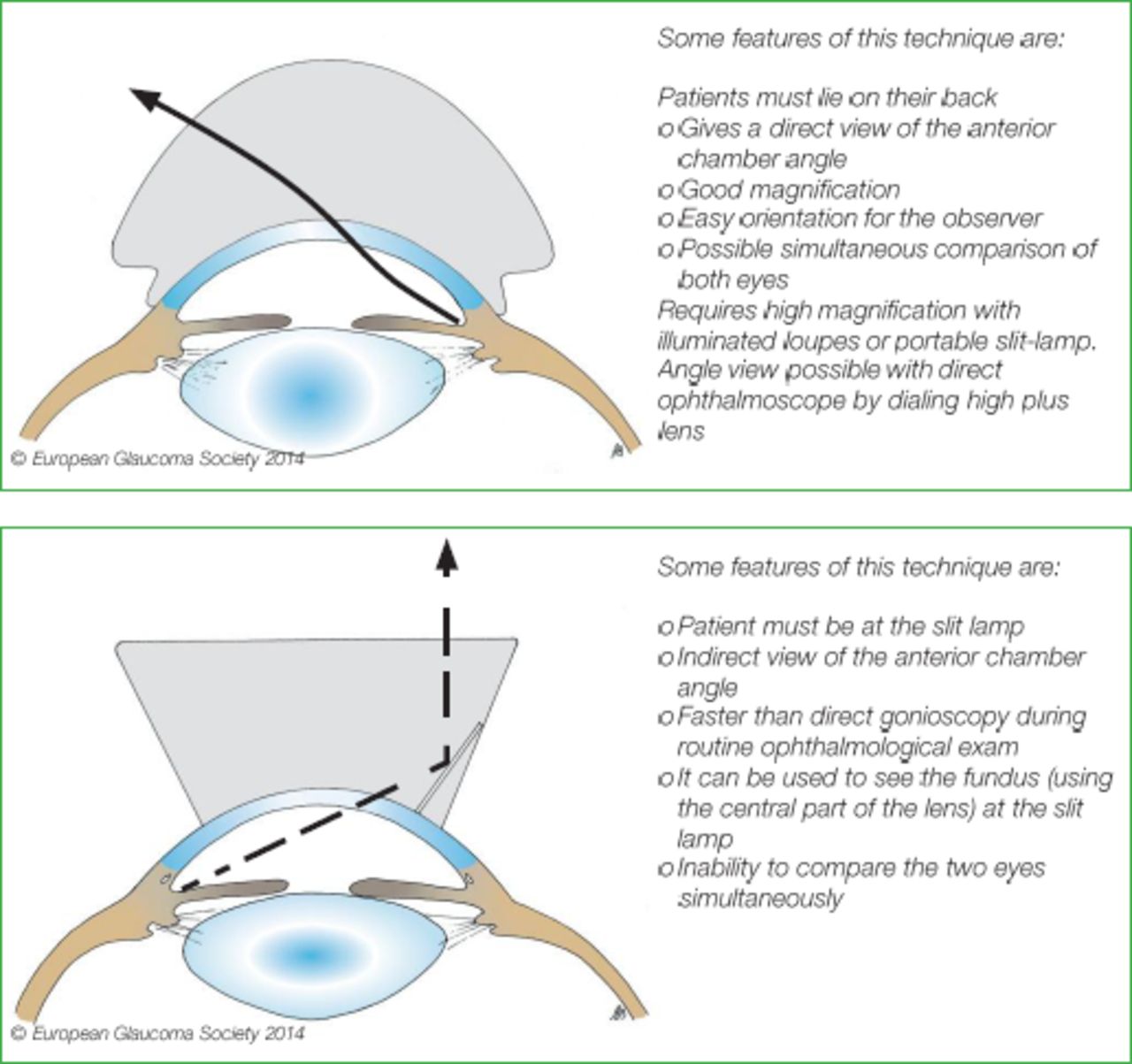
Direct Gonioscopy
The use of some contact goniolenses like the Koeppe or Barkan lens permits the light from the anterior chamber to pass through the cornea so that the angle may be viewed (Fig. 1.3 top).
Indirect Gonioscopy
The light from the anterior chamber is made to exit via a mirror built into a contact glass (Fig. 1.3. bottom).
The most common Gonioscopy lenses:
Influence of corneal status, thickness and tear film on the intraocular pressure (IOP) value measured with the Goldmann Applanation Tonometry.
1.2.2.1 ‘Dynamic indentation’ gonioscopy
It is recommended to use a small diameter lens for indentation (e.g.: 4-mirror) [I,D]. When gentle pressure is applied by the lens on the center of the cornea, the aqueous humour is pushed back. In appositional angle-closure, the angle can be re-opened. If there is adhesion between the iris and the meshwork, as in goniosynechiae, that portion of angle remains closed (Fig. 1.4(3)).
When pupillary block is the prevalent mechanism the iris becomes peripherally concave during indentation. In iris plateau configuration this iris concavity will not be extended by indentation to the extreme periphery, which is a sign of anteriorly placed ciliary processes (double hump sign). When the crystalline lens has a particularly prominent role, indentation causes the iris to move only slightly backwards, retaining a convex profile (Fig. 1.4(4)).
To differentiate appositional from synechial closure “indentation” or “dynamic” gonioscopy is essential.

Dynamic indentation gonioscopy. When no angle structure is directly visible before indentation, angle-closure may be present, and it can be synechial or appositional (1). If during indentation the iris moves peripherally backwards and the angle recess widens (2), the picture in (1) is to be interpreted as appositional closure and a suspicion of relative pupillary block is raised (2). When during indentation the angle widens but iris strands remain attached to the angle outer wall (3), the picture in (1) is to be interpreted as synechial closure. A large and/or anteriorly displaced lens causes the iris to move only slightly and evenly backwards during indentation (4) making the lens a likely component of angle-closure.
1.2.2.2 Gonioscopy technique without indentation
With indirect Goldmann-type lenses it is preferable to start by viewing the inferior angle, which often appears wider than the superior angle, because it is easier to identify the different structures. Then to continue rotating the mirror [II,D]. The anterior surface of the lens should be kept perpendicular to the observation axis so that the appearance of the angle structure is not changed as the examination proceeds. The four quadrants are examined by a combination of slit-lamp movements and prism rotation.
In case of a narrow approach, it is possible to improve the visualization of the angle recess by asking the patient to look in the direction of the mirror being used.
Practical points
Related to the technique
Gonioscopy should be performed in a dark room and with a small slit beam [I,D]. The most widely used technique is indirect gonioscopy where the angle is viewed in a mirror of the lens. The position of the globe is of importance. Angle width grading must be performed with the eye in primary position to avoid misclassification. If the patient looks in the direction of the mirror the angle appears wider and vice versa. A second pitfall is inadvertent pressure over the cornea, which will push back the iris, and gives an erroneously wide appearance to the angle. This occurs when the diameter of the lens is smaller than the corneal diameter e.g.: 4-mirror lenses. With a large diameter goniolens, indentation is transmitted to the periphery of the cornea distorting the angle.
Related to the anatomy
Recognition of angle structures may be impaired by variations in the anterior segment structures like poor pigmentation, iris convexity or existence of pathological structures.
Pharmacological mydriasis
Dilation of the pupil with topical or systemic drugs can trigger angle-closure. Angle-closure attacks can occur, even bilaterally, in patients treated with systemic parasympatholytics before, during or after abdominal surgery and has been reported with many systemic drugs such as serotonergic ‘appetite’ suppressants53.
Although pharmacological mydriasis with topical tropicamide and neosynephrine is safe in the general population even in eyes with a narrow approach, IOP elevation can occur in occasional patients (approx. 10%)54. Screening with van Herick’s test can detect angles at risk prior to dilating (Fig. 1.6).
Systemic drugs with effects on the angle
Theoretically, although any psychoactive drugs have the potential to cause angle-closure, it is unlikely that pre-treatment gonioscopy findings alone are of help to rule out such risk. In eyes with narrow angles, it makes sense to repeat gonioscopy and tonometry after initiation of treatment [II,D]. Prophylactic laser iridotomy needs to be evaluated against the risks of angle-closure or of withdrawal of the systemic treatment [II,D]. (See Ch. 2.4). None of these drugs is contraindicated per se in open-angle glaucoma. Ciliochoroidal detachment with bilateral angle-closure has been reported after oral sulpha drugs and topiramate55.
1.2.3 Grading
The use of a grading system for gonioscopy is highly desirable48, 56, 57 [I,D]. It stimulates the observer to use a systematic approach in evaluating angle anatomy, it allows comparison of findings at different times in the same patients, or to classify different patients.
The Spaeth gonioscopy grading system is the most detailed (Fig. 1.5) 48.
Other practical grading systems are those of Shaffer58 and Kanski59; both are based on angle width and visibility of the structures.

The Spaeth Grading System of gonioscopy finding.

The Van Herick test.
1.2.3.1 Slit lamp-grading of peripheral AC depth - The Van Herick Method
The Van Herick grading is an important part of any comprehensive eye examination (Fig. 1.6) [II,D]. This method is very useful if a goniolens is not available57, 60 [I,D] and can identify the need for gonioscopy in patients not otherwise suspected of glaucoma but it is not a substitute for gonioscopy. This technique is based on the use of corneal thickness as a unit measure of the depth of the anterior chamber at the furthest periphery, preferably on the temporal side.
Grade 0 represents iridocorneal contact.
A space between iris and corneal endothelium of < 1/4 corneal thickness, is a Shaffer grade I. When the space is ≥ 1/4 < 1/2 corneal thickness the grade is II. A grade III is considered not occludable, with an irido/endothelia l distance ≥ 1/2 corneal thickness.
1.2.4 Anterior Segment Imaging Techniques
UBM, anterior segment OCT and Scheimpflug cameras can be useful in some circumstances. Added to gonioscopy, these techniques help elucidate the mechanism of angle-closure in many cases [II,D]. Due to their limited availability and costs however, they are applied to cases which are most difficult to interpret61-69. UBM is very helpful in diagnosis behind the iris and the pigmented epithelium (tumours, cysts). Anterior segment OCT and Scheimpflug cameras are suitable for volumetric measurements and documentation of the dynamics of the chamber angle at different light conditions. These instruments currently give information only on the examined sector and not about the total circumference. None of these imaging methods provides sufficient information about the anterior chamber angle anatomy to be considered a substitute for gonioscopy70-89
1.3 - Optic Nerve Head and Retinal Nerve Fibre Layer
Glaucoma changes the appearance of the optic nerve head (ONH) and the retinal nerve fibre layer (RNFL) in a characteristic fashion.
Contour changes can best be appreciated with a magnified stereoscopic view. Therefore the initial examination, and follow-up examinations for contour change, should be made preferably through a dilated pupil [I,D]. Interim examinations, aimed at detecting striking features such as disc haemorrhages, may be performed through an undilated pupil stereoscopic examination of the posterior pole is best performed with a:
Indirect non-contact fundus lens with sufficient magnification at the slit-lamp or
Direct contact fundus lens at the slit-lamp
The direct ophthalmoscope is also useful for ONH and RNFL examination. Although three-dimensional information using parallax movements is possible, binocular examination through a dilated pupil is superior. The clinical evaluation of the ONH and RNFL should assess the following features [I,D].
1.3.1 Clinical Examination - Qualitative
1.3.1.1 Neuroretinal Rim
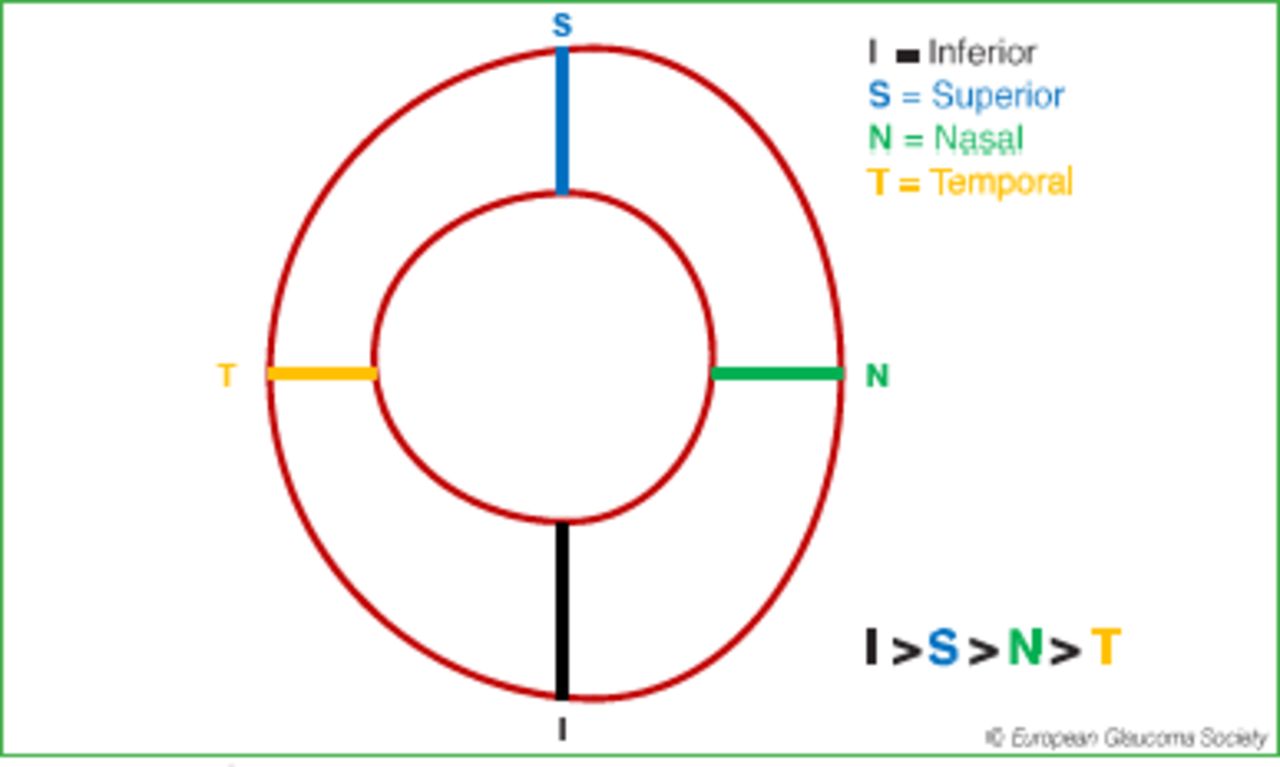
In a healthy eye, the shape of the rim is influenced by size, shape and tilting of the optic nerve head. The disc is usually slightly vertically oval, often more so in black subjects who may also have larger discs. In normal sized discs, the neuroretinal rim is typically at least as wide at the 12 and 6 o’clock positions as elsewhere and usually widest (83% of eyes) in the infero-temporal sector, followed by the supero-temporal, nasal and then temporal sectors (the ‘ISNT’ rule, see fig. 1.10)90.
This pattern is less obvious in larger discs, in which the rim is distributed more evenly and in a smaller discs where cupping may not be evident. Larger and a smaller discs are harder to interpret: e.g., in small discs the changes associated with glaucoma may not result in cupping, but ‘saucerization’ of the disc surface instead, and in large optic discs the normal rim is relatively narrow and can potentially be misinterpreted as glaucomatous.
The exit of the optic nerve from the eye may be oblique, giving rise to a tilted disc. Tilted discs are more common in myopic eyes, and show a wider, gently sloping rim in one disc sector and a narrower, more sharply-defined rim in the opposite sector. Discs in highly myopic eyes are even harder to interpret.
Glaucoma is characterized by progressive narrowing of the neuroretinal rim. The pattern of rim loss varies and may take the form of diffuse narrowing, localized notching, or both in combination (Fig. 1.7). Narrowing of the rim, while occurring in all disc sectors, is generally more common and greatest at the inferior and superior poles91-95

Progression of glaucomatous damage at the optic disc:
Early localized loss (A1), advancing to localized plus diffuse rim loss (A2).
Early localized rim loss, polar notches (B1); more advanced polar notches (B2). Diffuse or concentric rim loss, early (C1); advanced (C2).
Diffuse rim loss (D1), followed by localized r im loss (notch) (D2).
1.3.1.2 Retinal nerve fibre layer
The RNFL appearance is best assessed with a red-free (green) photograph. Clinically, the RNFL can be assessed with the red-free light or a short, narrow beam of bright white light at high magnification to explore the parapapillary region. In healthy eyes, smaller retinal vessels are embedded in the RNFL. The RNFL surface is best seen if the focus is adjusted just anterior to the retinal vessels.
The fibre bundles are seen as silver striations. About two disc diameters from the disc the RNFL thins and feathers out. Slit-like, groove-like, or spindle-shaped apparent defects, narrower than the retinal vessels, may be seen in the normal fundus. The RNFL becomes less visible with age, and is more difficult to see in less pigmented fundi.
Defects are best seen within two disc diameters of the disc. Focal (wedge and slit) defects are seen as dark bands, wider than retinal vessels and extending from the disc margin, unless obscured by vessels. These focal defects are more easily seen than generalized thinning of the RNFL, which manifests as a loss of brightness and density of striations. When the RNFL is thinned, the blood vessel walls are sharp and the vessels appear to stand out in relief against a matt background. The initial abnormality in glaucoma may be either diffuse thinning or localized defects. Since the prevalence of RNFL defects is < 3% in the normal population, their presence is likely to be pathological96-98.
1.3.1.3 Optic disc haemorrhages
The prevalence of small (‘splinter’) haemorrhages on or bordering the optic disc has been estimated to be ≤ 0.2% in the normal population99. On the other hand, a large proportion of glaucoma patients have optic disc haemorrhages (ODHs) at one time or another (Fig. 1.8). They are very often overlooked at clinical examinations, and are easier to find in photographs100-103. Many studies have shown that ODHs are associated with disease progression.

Optic disc haemorrhage.
1.3.1.4 Vessels at the optic disc
Narrowing of the neuroretinal tissue will change the position of the vessels at the optic disc with bending, bayoneting or baring of circumlinear vessels. Those positional changes are particularly important to observe when looking for progression, in comparison to a baseline photo.
1.3.1.5 Parapapillary atrophy
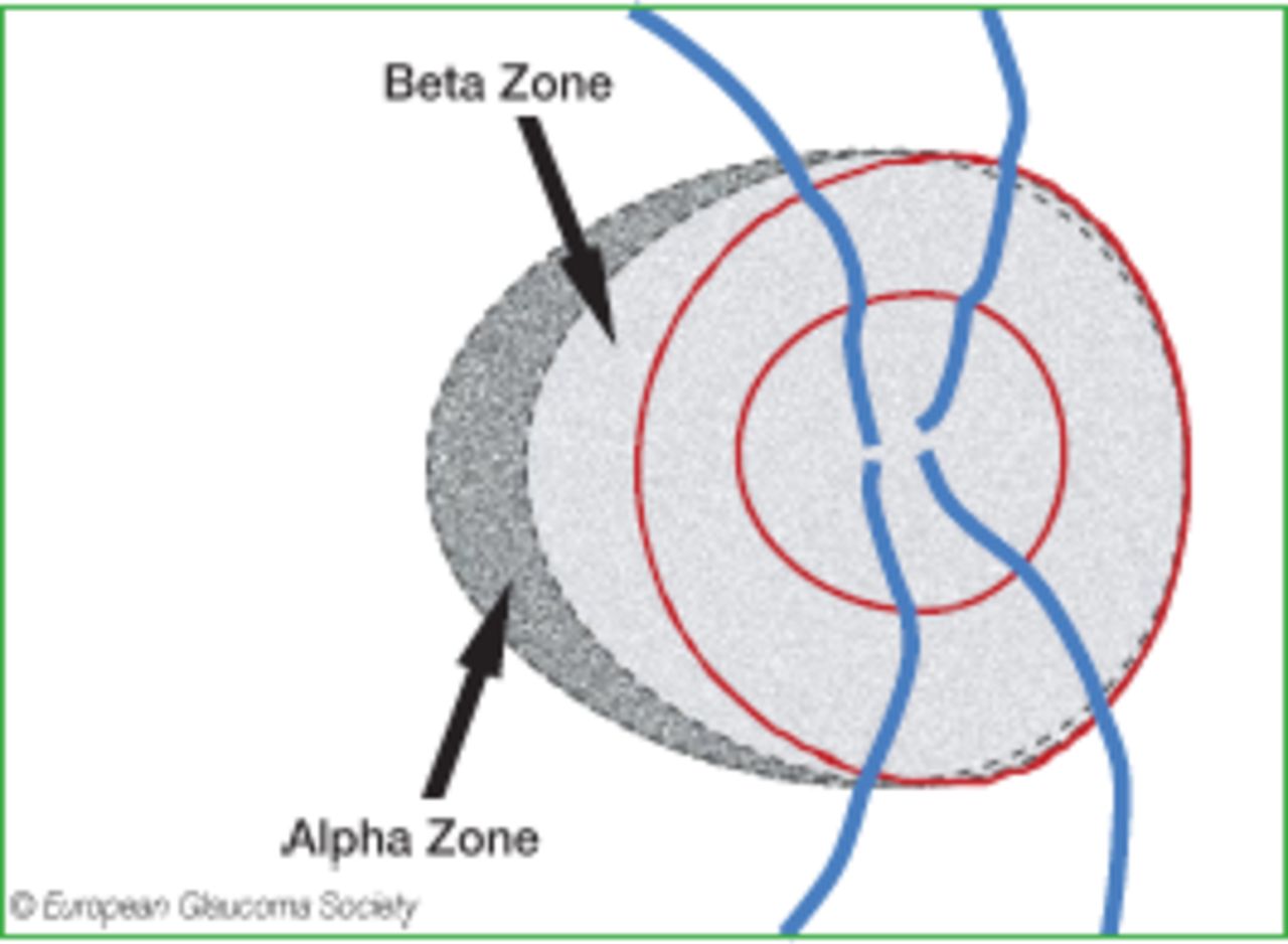
Parapapillary atrophy can be differentiated into an Alpha zone, which is present in almost any eye, and into a Beta zone, which is present in approximately 25% of normal eyes and in a significantly higher percentage of eyes with glaucoma104-106.
The Alpha zone has been defined as irregular hyperpigmentation and hypopigmentation and it is located in the periphery of parapapillary atrophy. The Beta zone is characterized by visible sclera and visible large choroidal vessels and a location between the peripapillary ring and Alpha zone. Both zones are usually located at the temporal margin of the optic disc, more often in the inferotemporal region than in the superotemporal region. Histologically, the Alpha zone corresponds to irregularities in the retinal pigment epithelium, and the Beta zone shows a complete loss of retinal pigment epithelium, an almost complete loss of photoreceptors and a closure of the choriocapillaris. The Beta zone may be associated with a greater amount of glaucomatous optic neuropathy and a higher risk of further progression of glaucoma107. The location of the Beta zone outside the optic disc spatially correlates with the location of the most marked loss of neuroretinal rim inside of the optic disc, together with the longest distance to the central retinal vessel trunk in the optic nerve head104. In clinical routine, a large ophthalmoscopical Beta zone (in particular in non-myopic eyes) should be regarded as an extra clue, and not as a definite sign of glaucoma (Fig. 1.9) [I,C].

ONH with parapapillary atrophy. The Alpha zone is located peripheral to beta zone, and is characterized by irregular hypo-and hyperpigmentation. The Beta zone of atrophy is adjacent to the optic disc edge, external to Elschnig’s ring (a white circular band that separates the intra-from the peri-papillary area of the optic disc), with visible sclera and large choroidal.
1.3.1.6 The ISNT rule
In normal eyes with a normal optic disc shape, with a greater vertical diameter, the neuroretinal rim shows a characteristic shape: it is usually widest at the inferior disc pole, followed by the superior disc pole, the nasal disc region, and finally the temporal disc region108. For mnemonic reasons, this sequence of disc sectors was abbreviated as “ISNT” (Inferior-Superior-Nasal-Temporal) rule. In many eyes, the rim can be wider superiorly than inferiorly, however in almost all normal eyes the rim is smallest in the temporal 60° of the optic nerve head (Fig. 1.10). The most important letter in the “ISNT”-rule is therefore the “T”. The application of the ISNT rule is helpful for detecting early glaucomatous optic nerve damage, since in the early stage of glaucoma, the rim gets smaller preferentially in temporal inferior disc region or the temporal superior disc region, leading to a rim shape in which the rim can be equal in width in the inferior or superior region as compared with the temporal region. For the assessment of the ISNT rule, it is important to consider that the area of the peripapillary ring does not belong to the neuroretinal rim. It holds true in particular for the temporal disc region.

The ISNT rule.
1.3.2 Clinical Examination - Quantitative
1.3.2.1 Optic disc size (vertical disc diameter)
The optic disc size greatly varies in the population. The width of the rim and, conversely, the size of the cup, vary with the overall size of the disc. The mean vertical disc diameter is approximately 1.5 mm109.
The vertical diameter of the optic disc can be measured at the slit lamp using a handheld high power convex lens. The slit beam should be coaxial with the observation axis; a narrow beam is used to measure the vertical disc diameter using the inner margin of the white Elschnig’s ring as the reference. A correction factor needs to be used depending on the magnification of the handheld lens (Fig. 1.11).

Optic disc size assessed at the slit lamp with handheld high power convex lens.
1.3.2.2 Rim Width and Cup/Disc ratio
A large Cup/Disc Ratio (CDR) has been used as a sign of glaucoma damage. However, the CDR depends on the disc size, and a large CDR in normal large discs may be erroneously considered glaucomatous and a small CDR in glaucomatous small discs may be erroneously considered as normal110 (Fig. 1.12). The use of CDR to classify patients is not recommended and the attention should be focused on the disc rim [I,D].
In healthy eyes, cupping tends to be symmetrical between the two eyes, the vertical CDR difference being less than 0.2 in over 96% of normal subjects. A difference in CDR between eyes with equal optic disc size is suggestive of acquired damage and glaucoma.
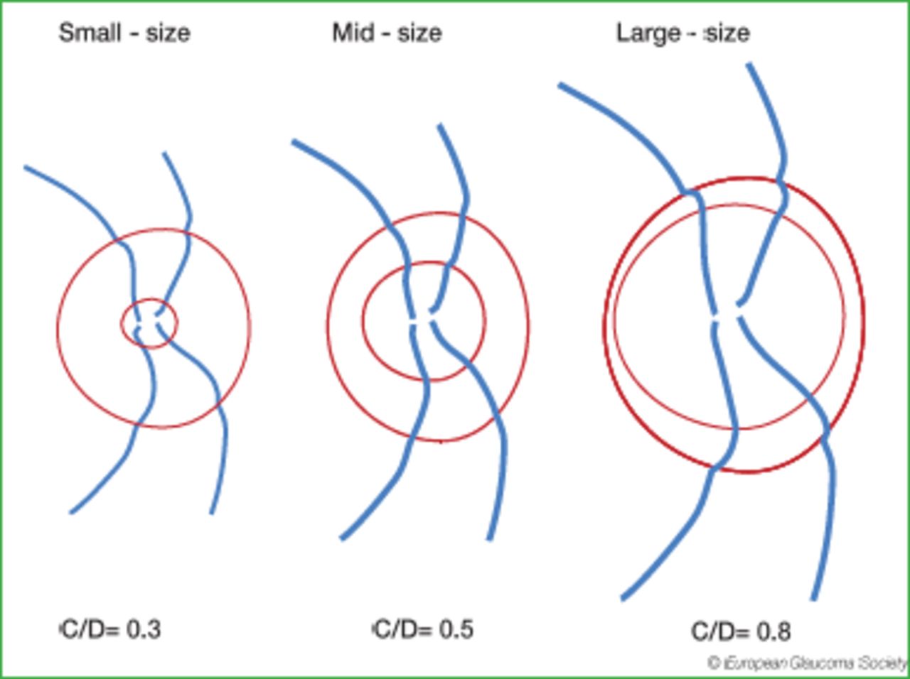
Optic nerve heads with different disc areas but with the same rim area and the same number of retinal nerve fibres: small size disc (disc area less than 2 mm² and C/D=0.3), mid-size disc (disc area between 2 and 3 mm², C/D=0.5) and large disc (disc area greater than 3 mm² and C/D=0.8).
1.3.3 Recording of the Optic Nerve Head (ONH) Features
At baseline, some form of imaging is recommended to provide a record of the ONH appearance [I,D]. If colour photos are not available, a detailed manual drawing is recommended. Even if it is difficult to draw a good picture of the ONH, the act of making a drawing encourages a thorough clinical evaluation of ONH [II,D].
Stereoscopic is preferred to non-stereoscopic photography [I,D]. Colour photography with a 15° field gives optimal magnification. Sequential photographs can be used to detect progression of optic disc damage.
1.3.3.1 Quantitative Imaging
Quantitative imaging of the optic nerve head, retinal nerve fibre layer and inner macular layers have been widely used to assist glaucoma diagnosis and to detect glaucomatous progression during follow-up.
1.3.3.2 Classification
For cross sectional classification, imaging instruments typically provide three potential outcomes: “within normal limits”, “borderline” and “outside normal limits”. No imaging device provides a clinical diagnosis but just a statistical result, based on comparison of the measured parameters with the corresponding normative database of healthy eyes. Therefore an interpretation of the result in the context of all clinical data is mandatory [I,D]. The clinician should also assess the quality of the image and analysis and judge whether the normative database is relevant for the particular patient before including the classification in the assessment of the patient [I,D]. For instance, imaging artefacts and software errors are quite common and more frequent in eyes that are highly myopic or have very tilted nerves, and few devices have normative data appropriate to these eyes. The various imaging technologies have their own advantages and limitations, and their classification shows only partial agreement in early glaucoma111. In addition, agreement between classification with quantitative imaging and visual field testing is only moderate in early glaucoma.
1.3.3.3 Detection of progression
Most commercial imaging devices have software for quantifying glaucomatous progression, including the rate of progression. The classification algorithms described above should not be used to assess progression [I,D]. In general, normative databases are not needed for progression analysis because the patient’s baseline images provide the reference for change. High quality baselines images are, therefore, of considerable importance. The user should assess the test series for the quality of images and software analysis before including the software output in the assessment of the patient [I,D]. Agreement between structural progression and functional deterioration, over the relatively short duration of reported studies, is only partial or poor112, 113.
Provided the images in a series are of good quality and progression analysis is
consistent over several tests, imaging devices provide useful data, additional to those gained from visual field testing, concerning a patient’s glaucoma damage.
1.3.3.4 Imaging instruments
A complete list of all available technologies is beyond the scope of the guidelines.
Heidelberg Retina Tomography (HRT)
The Heidelberg Retina Tomograph (Heidelberg Engineering, Heidelberg, Germany) is used to profile and measure the three-dimensional anatomy of the optic nerve head and surrounding tissues. It can also detect progressive changes in optic nerve head surface topography. To classify an optic nerve head, three methods can be used: the Moorfields Regression Analysis (MRA), the linear discriminant analysis formulas and the Glaucoma Probability Score (GPS)114-116. The classification algorithms tend to over-report ‘outside normal limits’ in large optic discs. For progression analysis, the software provides a map of surface height changes compared to baseline (Topographic Change Analysis [TCA]); the area and volume of changing regions is presented as a plot over time. Graphs of rim area over time are also available.
Scanning laser polarimetry (GDx-ECC)
The GDx-ECC instrument (Carl Zeiss Meditech Inc., Dublin, CA, USA) measures retinal nerve fibre layer thickness around the optic nerve head on the basis of retardation of the illuminating laser light. All polarizing structures in the eye cause retardation, especially the cornea. With Enhanced Corneal Compensation (ECC), polarization artefacts arising both from the anterior segment and behind the retina are attenuated117. The main parameter to help distinguish healthy subjects from glaucomatous patients is the NFI (nerve fibre indicator), although clinicians should also evaluate the distribution of the retinal nerve fibre layer around the optic disc (the ‘TNSIT’ curve). Trend and change from baseline analyses for progression are available.
Optical coherence tomography (OCT)
Optical coherence tomography is based on interferometry. Current instruments, Fourier-domain (FD) or Spectral domain (SD) and swept-source OCT systems, provide faster image acquisition, higher resolution and better image segmentation than time-domain OCT. Several companies produce FD/SD OCT instruments. Their technical, software and normative database characteristics vary; thus the values measured with different OCT systems are not interchangeable. Three main parameter groups are measured and analysed for classification and detection of progression: Optic Nerve Head, Retinal Nerve Fibre Layer and Ganglion Cell Complex. In general, the optic nerve head parameters with OCT may be less informative than the retinal nerve fibre layer and the ganglion cell complex parameters118. To identify and measure glaucomatous progression with OCT systems trend analysis of the retinal nerve fibre layer thickness and inner macular retinal thickness parameters are particularly useful119.
How to use imaging at baseline [II,D]
Glaucoma suspects with normal or unreliable visual field Glaucoma with early and moderate damage
How to use imaging for monitoring progression [II,D]
Frequency should be similar to that for VF testing
Patients should be followed with the same test/method to facilitate estimation of progression [I,D].
Baseline, repeated within 3 months after baseline, and then up to 4 more times in the first two years in case of high risk of progression [II,D].
Baseline, repeated annually, for ocular hypertensives [II,D].
Although knowing the test-retest variability would be indispensable in determining the optimal frequency of performing imaging tests, in every-day clinical work it seems currently impossible to take into account the large number of parameters and their largely variable reproducibility nor to verify the cost effectiveness of imaging for glaucoma120.
1.4 - Perimetry
1.4.1 Perimetry Techniques
Visual field testing is important for the diagnosis of glaucoma, and even more important for follow-up and management of glaucoma [I,D].
A complete list of all available technologies and strategies is beyond the scope of the guidelines.
1.4.1.1 Computerised and manual perimetry
Static computerised perimetry should be preferred in glaucoma management. Kinetic e.g. Goldmann perimetry is not suitable for detection of early glaucomatous field loss and small defects will often be lost between isopters121.
Computerised perimetry is also less subjective; the results are numerical and tools for computer-assisted interpretation are available. Manual kinetic perimetry may be helpful in patients who are unable to perform automated perimetry.
1.4.1.2 Standard Automated Perimetry - SAP
Glaucoma perimetry has become more standardised over time and today the term Standard Automated perimetry (SAP) is often used. SAP refers to static computerised threshold perimetry of the central visual field performed with white stimuli on a dimmer white background.
Test algorithms and programs
In glaucoma care threshold perimetry is the recommended standard [I,D]. Commonly used threshold algorithms are: ‘SITA Standard’ and ‘SITA Fast’ in the Humphrey perimeter. SITA Fast has the advantage of reduced test time but this may come at the cost of increased variability. In the Octopus perimeter the commonly used threshold algorithms called the ‘Dynamic Strategy’. TOP algorithm is more rapid, but may have lower resolution than other threshold tests because threshold values are determined by averaging test results from several adjacent test point locations122.
Glaucoma perimetry is performed using a Goldmann size III stimulus in the central 25–30° field where the great majority of retinal ganglion cells are located [I,D].
Common test point patterns are the identical 30-2 and 32 test point patterns of the Humphrey and Octopus perimeters respectively and G1 and G2 patterns of the Octopus, which cover the central 30°. A commonly used pattern is the 24-2 pattern of the Humphrey perimeter, which covers a somewhat smaller area and thereby reduces test time. Only a small amount of information is lost if the smaller patterns are used as compared to the larger ones, and common test artefacts from, e.g., trial lens rims or droopy lids are less common with the more central patterns.
Selecting a test
It is recommended that clinicians select and familiarise themselves with suitable SAP tests. Patients should be followed with the same test to facilitate estimation of progression [I,D]. For those with very advanced disease it may be necessary to consider using a Goldmann size V stimulus rather than size III, or a perimetric strategy which focuses more closely on the remaining area of visual field. In both perimeters one may use test point patterns covering only the central 10° of the field in eyes which have only ‘tunnel’ fields left, e.g. the Octopus M1 or M2 or the Humphrey 10-2 [I,D].
The Humphrey Field Analyzer and the Octopus perimeter are the two most commonly used SAP perimeters in Europe. Other less frequently used SAP perimeters also having threshold programmes are available.
1.4.1.3 Non-conventional perimetry
Other modalities of computerised perimetry use different stimuli to SAP. Examples are SWAP (Short Wavelength Automated Perimetry), FDT (Frequency Doubling Technology), HEP (Heidelberg Edge Perimetry) and HRP (High-pass resolution perimetry or ring perimetry) and flicker perimetry. There is insufficient evidence that these tests offer any advantage over SAP123-126.

Consider the reliability of the test before making decisions based on it.
1.4.1.4 Patient instructions
The role of the operator is of great importance. To patients who are naive to the test, the operator must explain what to expect and how to react to stimuli. The operator needs to be in the vicinity of the perimeter to react to any patient queries [I,D]. A quiet, dimly lit environment should be ensured. A short demonstration, before the actual test starts, will also help patients understand the test. The operator should have taken the tests to better understand the experience of taking the test. It should be explained that most stimuli will be very dim and even patients with normal visual fields will be expected to ‘miss’ many stimuli [II,D].
1.4.2 Interpreting test results
1.4.2.1 Printouts
Humphrey and Octopus both provide similar statistical analyses of single field test results presented on printouts containing maps of the visual field plus visual field indices and other means of interpreting a test result.
The numerical threshold map provides the ‘raw’ estimated threshold values a teach test point location.
The grey scale or colour coded map provides a graphical representation of the numerical threshold map.
The numerical total deviation map shows point-wise differences between the age-corrected normal threshold value at each test point location and the measured value.
The numerical pattern deviation map shows the same values but after correction for diffuse loss of sensitivity. Thus, it highlights focal loss of sensitivity.
Probability maps provide the statistical significance of the numerical deviations.
1.4.2.2 Reliability indices
These indices are meant to estimate patient reliability. With proper instructions almost all patients are able perform reliable tests.
High frequencies of false positive answers (FP), are clearly a sign of poor reliability, but high frequencies of false negatives (FN) are of relatively little value. High rates of fixation losses (FL) may indicate poor attention to the fixation target. In most modern perimeters patients’ fixation is continuously monitored during the test by an automatic eye/gaze tracker.
The operator has an important role in monitoring in assessing the reliability of the test as it is performed and informing the clinician e.g. by annotating the test result if necessary.
1.4.2.3 Visual field indices
Visual field indices are numbers summarising perimetric test results. An useful index is MD (mean defect in the Octopus system or mean deviation in the Humphrey system). MD represents the average difference between normal age-corrected sensitivity values and the measured threshold values at all test point locations. A new index developed for the Humphrey perimeter is VFI, which is similar to the MD value but more centrally weighted, expressed in percent rather than in decibels and more resistant to diffuse loss127, 128.
The global indices include PSD (Humphrey) and LV (Octopus) measure the local spatial variability of the visual field. PSD and LV can be used for diagnosis, but they are less informative than the probability maps. Software to produce graphs mapping visual field loss to expected anatomical regions is available.
1.4.2.4 Recording the visual field indices
A simple method to record serial data from VF is the GSS; this will give a visual overview, without any statistical support 129, 130
1.4.2.5 Summarising diagnostic features
The Glaucoma Hemifield Test (GHT)
The Glaucoma Hemifield Test is incorporated in the Humphrey perimeter. This analysis classifies results as ‘within normal limits’, ‘outside normal limits’ or ‘borderline’. The classification of outside normal limits is designed to identify glaucoma. Two more GHT classifications are ‘general depression of sensitivity’ and ’abnormally high sensitivity which goes hand in hand with high frequencies of FP responses’.
The Bebié curve
The Bebié curve or the cumulative defect curve in the Octopus system is a summary graph of localised and diffuse sensitivity loss. In entirely diffuse loss the curve of the measured sensitivities is lower than but parallel to the displayed normal curve. In focal loss the right part of the measured curve is depressed as compared to the normal reference curve.
D iagno sis ba s e d on cluste re d p oints
Clustered test point locations with significantly reduced sensitivity are more reliable indicators of early glaucomatous field loss than scattered points. A rule, which is of ten used to classif y a test result as glaucomatous, stipulates a minimum of three clustered points with significantly depressed sensitivity, of which one should have a significance of p<1% [I,D]. Usually, the test point locations immediately surrounding the blind spot are ignored in this analysis.
1.4.2.6 Confirmation of classification
Field defects which appear clearly glaucomatous and fit with the clinical picture may not need confirmation to support a diagnosis [I,D]. Visual fields with subtle defects may require confirmatory tests. (See FC IV).
The learning effect.
Many subjects show an improvement in performance reflected as improved reliability and sensitivity over the first few tests.

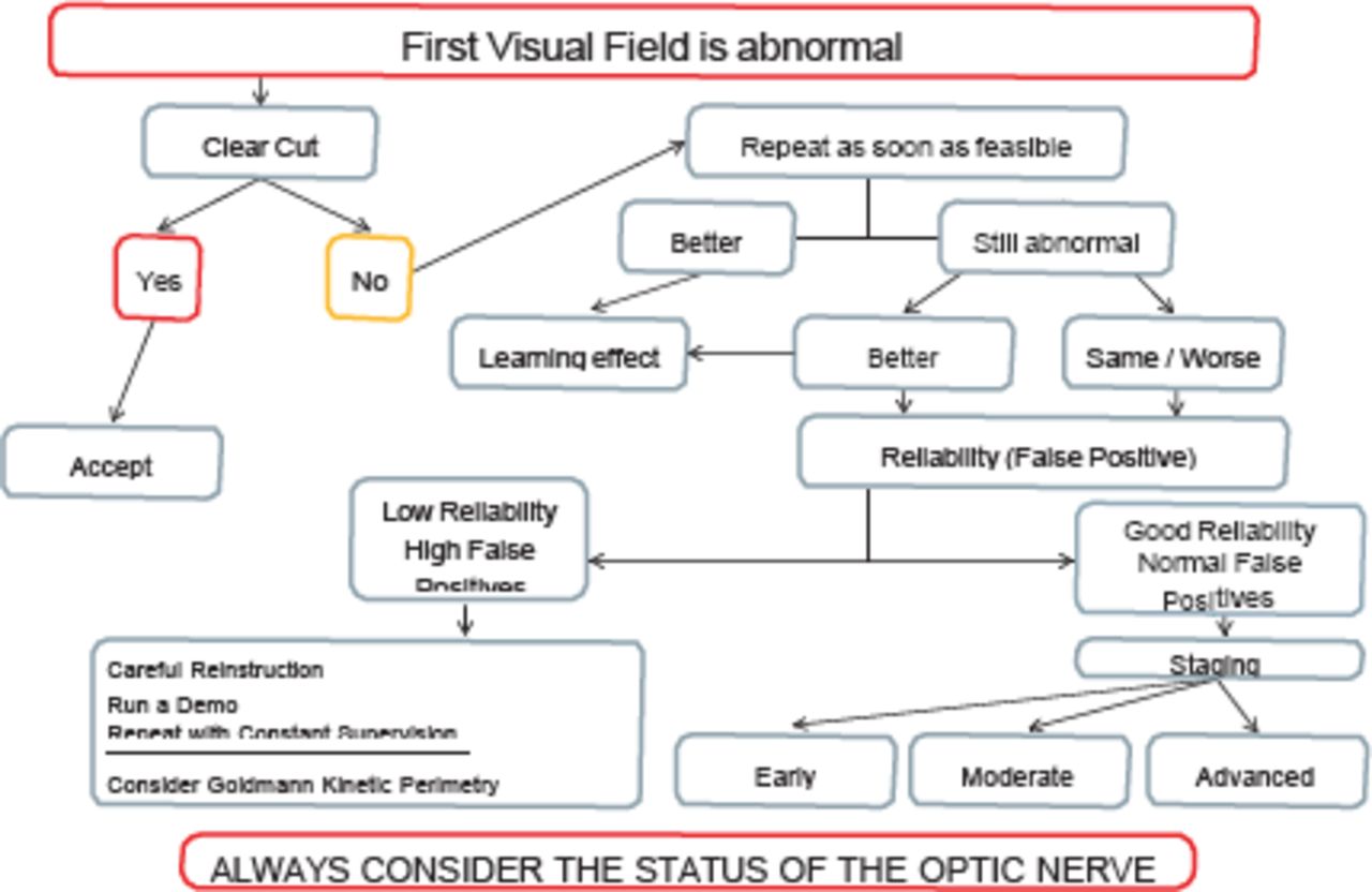
FC IV - Diagnostic strategy when initial visual Field is abnormal
1.4.2.7 Assessing progression
In follow-up it is important to know whether the visual field of an eye is deteriorating and the rate of progression [I,D]. When assessing change from baseline, apparent progression needs to be confirmed in two or more tests [I,D].
There are two main approaches to computer-assisted progression analyses:
Event analyses (designed to answer the question of whether the field has progressed) With Glaucoma Change Probability Maps (GCPMs) all visual field tests are compared to baseline consisting of an average of two baseline tests. Test point locations that have deteriorated more than the expected test-retest variation are flagged. Eyes that show deterioration of at least three test point locations are flagged as possibly progressing if the finding is repeated in two consecutive tests and likely progressing if existing in three consecutive tests. The rules used in EMGT131 are part of the HVF Analyser’s guided progression analyses (GPA) program.
2. Trend analyses (quantify the rate of progression)
The perimetric rate of progression is the velocity of worsening of the visual field, and is usually measured by performing linear regression analysis of the MD index or the newer VFI index over time. With MD rate of progression is expressed in dB/year, and with VFI in %/year.
Trend analysis of global indices includes linear regression of MD and VFI for the Humphrey and linear regression of MD, LV, DD and LD for the Octopus. The Octopus provides trend analysis of functionally related clusters of test points. Several stand-alone software programs are available to perform trend analysis of individual test locations, clusters or global indices, depending on the product. These include Peridata, PROGRESSOR and Eye Suite. Some of the systems described above use trend data to try to predict the future status of the visual field.
1.4.2.8 Number of tests
Commonly used event and trend analyses require at least five and preferably more tests to detect progression. However in some cases progression may be detected before this. This demonstrates the need for relatively frequent perimetry in those eyes where it is considered necessary to find early progression.
Determining the rate of progression of an individual eye requires a long enough time span (at least two years) and enough field tests. It is important to identify eyes showing a fast rate of progression at an early stage. Ideally, all newly diagnosed glaucoma patients should be tested with SAP three times per year during the first two years after diagnosis [II,D].
1.4.3 Staging of Visual Field Defects
When discussing disease stages in glaucoma, the status of the visual field is often used as the most important reference. A discrete-levels staging system132, modified from the Hodapp-Parrish classification133 has been in use for several years.
The GSS use a combination of MD and PSD to chart the stage of damage129, 130. Staging systems may be of great interest in scientific studies, cost studies et cetera, but they are of limited value in clinical management.
Ideally for glaucoma management one should be able to detect and quantify disease progression in small steps rather than identifying only the transition from one stage to the next [I,D].
The Hodapp Classification
EARLY GLAUCOMATOUS LOSS
MD < -6 dB
Fewer than 18 points depressed below the 5% probability level and fewer than 10 points below the p < 1% level
No point in the central 5 degrees with a sensitivity of less than 15 dB
MODERATE GLAUCOMATOUS LOSS
MD < -12 dB
Fewer than 37 points depressed below the 5% probability level and fewer than 20 points below the p < 1% level
No absolute deficit (0 dB) in the 5 central degrees
Only one hemifield with sensitivity of < 15 dB in the 5 central degrees
ADVANCED GLAUCOMATOUS LOSS
MD > -12 dB
More than 37 points depressed below the 5% probability level or more than 20 points below the p < 1% level
Absolute deficit (0 dB) in the 5 central degrees
Sensitivity < 15 dB in the 5 central degrees in both hemifields
References:
- 1.↵
- 2.↵
- 3.↵
- 4.↵
- 5.↵
- 6.↵
- 7.↵
- 8.↵
- 9.↵
- 10.↵
- 11.↵
- 12.↵
- 13.↵
- 14.↵
- 15.↵
- 16.↵
- 17.↵
- 18.↵
- 19.↵
- 20.↵
- 21.↵
- 22.↵
- 23.↵
- 24.↵
- 25.↵
- 26.↵
- 27.↵
- 28.↵
- 29.↵
- 30.↵
- 31.↵
- 32.↵
- 33.↵
- 34.↵
- 35.↵
- 36.↵
- 37.↵
- 38.↵
- 39.↵
- 40.↵
- 41.↵
- 42.↵
- 43.↵
- 44.↵
- 45.↵
- 46.↵
- 47.↵
- 48.↵
- 49.↵
- 50.↵
- 51.↵
- 52.↵
- 53.↵
- 54.↵
- 55.↵
- 56.↵
- 57.↵
- 58.↵
- 59.↵
- 60.↵
- 61.↵
- 62.↵
- 63.↵
- 64.↵
- 65.↵
- 66.↵
- 67.↵
- 68.↵
- 69.↵
- 70.↵
- 71.↵
- 72.↵
- 73.↵
- 74.↵
- 75.↵
- 76.↵
- 77.↵
- 78.↵
- 79.↵
- 80.↵
- 81.↵
- 82.↵
- 83.↵
- 84.↵
- 85.↵
- 86.↵
- 87.↵
- 88.↵
- 89.↵
- 90.↵
- 91.↵
- 92.↵
- 93.↵
- 94.↵
- 95.↵
- 96.↵
- 97.↵
- 98.↵
- 99.↵
- 100.↵
- 101.↵
- 102.↵
- 103.↵
- 104.↵
- 105.↵
- 106.↵
- 107.↵
- 108.↵
- 109.↵
- 110.↵
- 111.↵
- 112.↵
- 113.↵
- 114.↵
- 115.↵
- 116.↵
- 117.↵
- 118.↵
- 119.↵
- 120.↵
- 121.↵
- 122.↵
- 123.↵
- 124.↵
- 125.↵
- 126.↵
- 127.↵
- 128.↵
- 129.↵
- 130.↵
- 131.↵
- 132.↵
- 133.↵