Article Text

Abstract
Background Adaptive optics scanning light ophthalmoscopy (AOSLO) enables direct visualisation of the cone mosaic, with metrics such as cone density and cell spacing used to assess the integrity or health of the mosaic. Here we examined the interobserver and inter-instrument reliability of cone density measurements.
Methods For the interobserver reliability study, 30 subjects with no vision-limiting pathology were imaged. Three image sequences were acquired at a single parafoveal location and aligned to ensure that the three images were from the same retinal location. Ten observers used a semiautomated algorithm to identify the cones in each image, and this was repeated three times for each image. To assess inter-instrument reliability, 20 subjects were imaged at eight parafoveal locations on one AOSLO, followed by the same set of locations on the second AOSLO. A single observer manually aligned the pairs of images and used the semiautomated algorithm to identify the cones in each image.
Results Based on a factorial study design model and a variance components model, the interobserver study's largest contribution to variability was the subject (95.72%) while the observer's contribution was only 1.03%. For the inter-instrument study, an average cone density intraclass correlation coefficient (ICC) of between 0.931 and 0.975 was calculated.
Conclusions With the AOSLOs used here, reliable cone density measurements can be obtained between observers and between instruments. Additional work is needed to determine how these results vary with differences in image quality.
- Retina
- Imaging
- Anatomy
This is an Open Access article distributed in accordance with the Creative Commons Attribution Non Commercial (CC BY-NC 3.0) license, which permits others to distribute, remix, adapt, build upon this work non-commercially, and license their derivative works on different terms, provided the original work is properly cited and the use is non-commercial. See: http://creativecommons.org/licenses/by-nc/3.0/
Statistics from Altmetric.com
Introduction
The adaptive optics scanning light ophthalmoscope (AOSLO) enables non-invasive confocal reflectance imaging of the cone photoreceptor mosaic in the living human eye.1 ,2 From these images, it is possible to examine the health of the cone mosaic using metrics such as cone density3 and cell spacing.4 ,5 Such measurements could provide extremely sensitive biomarkers for early detection of retinal disease and tracking of the retinal response to therapeutic intervention. Numerous studies have provided new insights into a wide range of conditions in which changes in metrics of the cone mosaic correspond to clinically observed deficits as well as to changes detected using other diagnostic modalities.5–12 Central to these clinical applications of AOSLO is the ability to quantify the cone mosaic, which requires consistent identification of cells. Unfortunately, there are few studies assessing the repeatability and reliability of metrics of cone topography, which limits the clinical utility of these metrics.
Given that emerging multicentre studies may need to employ different AOSLO instruments and different graders, it is important to assess how the reliability is influenced by each of these two potential sources of error. Intra-instrument, semiautomated cone density analysis of AOSLO images from a young, healthy population has been demonstrated to have a repeatability of 2.7%, suggesting that the difference between two measurements for the same subject on that instrument would be less than this value in 95% of observations.13 On this same image set, a fully automated algorithm was shown to have comparable reproducibility with an average cone density intraclass correlation coefficient (ICC) of 0.989, indicating that 98.9% of the total variability is due to real differences between subjects.14 However, these studies represent a best-case scenario as these are high-quality samples from a healthy retina imaged on a single instrument. Even with equivalent optical designs, a different result is possible since numerous variables can affect image quality and thus the performance of any image analysis algorithm. Here we sought to determine the interobserver and inter-instrument reliability of cone density measurements.
Materials and methods
Subjects
All research followed the tenets of the Declaration of Helsinki, and study protocols were approved by the Institutional Review Boards at the Medical College of Wisconsin. Subjects provided informed consent after the nature and possible consequences of the study were explained. Axial length measurements were obtained from all of the subjects using an IOL Master (Carl Zeiss Meditec, Dublin, California, USA) to calculate the scale of the retinal images.
To test interobserver reliability, 30 subjects with no vision-limiting pathology (19 males and 11 females, aged 25.1±5.7 years) were imaged (table 1). Twenty-one of the subjects previously participated in an earlier study.13 As a result, only nine new subjects were prospectively recruited and imaged for this part of the study.
Subject demographics
To assess inter-instrument reliability, 20 visually normal subjects (12 males and 8 females, aged 25.0±2.7 years) were recruited, 4 of whom also participated in the interobserver study (table 1). The 20 subjects were chosen to closely reflect the true heterogeneity in the population regarding parafoveal cone density. This is important because reliability is highly dependent on not only the magnitude of measurements errors but also on the heterogeneity in the population in which measurements are made.15 Based on an n=20, we calculated the expected CIs at different ICC values and observed narrow CIs for ICC values that would be what studies typically consider to be reliable. For comparison, studies on the reliability of OCT nerve fibre layer thickness measurements report having reliable measurements with ICC values of 0.4–0.5.16 ,17
Reflectance confocal AOSLO imaging of the photoreceptor mosaic
A previously described AOSLO was used to image the parafoveal cone mosaic of one eye of each subject.2 ,18 The wavelength of the super luminescent diode used for retinal imaging was 775 nm, subtending a field of view of about 1×1°. In the interobserver portion of the study, each subject’s head was stabilised using a chin and forehead rest. There was no pupil dilation or control of accommodation using eye drops. Three image sequences of 150 frames each were acquired at a single parafoveal location, approximately 0.65° from the centre of fixation. For this study, the image sequences for a given subject were acquired by the same operator; however, different operators were used for different subjects.
In the inter-instrument part of the study, image sequences of 150 frames were acquired at 8 parafoveal locations approximately 0.65° from the centre of fixation. After imaging the eight locations on one AOSLO, the subject was imaged on the second AOSLO at the same retinal locations. Data were analysed as right-eye equivalents. Each subject was stabilised using a dental impression on both devices. All subjects were imaged in consecutive sessions except for two (AD_1193, JC_10023) who needed to be imaged on separate days with the two devices due to scheduling difficulties. The same operators were used when collecting the images on the two AOSLO systems. The two AOSLO systems used here were of nearly identical optical design, with the system design having been previously reported.18
Analysing the cone mosaic
All image sequences were processed using a previously described strip registration method,19 generating a single 8-bit monochrome image per image sequence for subsequent analysis. The interobserver image set consisted of 90 images (30 subjects, 3 images per subject). The three images for a given subject were acquired from the same retinal location (∼0.65° from fixation) and aligned to one another using the strip registration approach. This ensured that the three images to be analysed for each subject were from exactly the same retinal location. The central 85×85 μm area of each image was then cropped for analysis. A previously described semiautomated programme was used to identify the cones in each image.13 After automated identification of the majority of cones in the image, the observer then reviewed each image and manually identified cones they deemed to be missed by the algorithm or removed cones they deemed to be selected in error by the algorithm. The user interface for the manual correction step is shown in figure 1. During the manual correction step, the brightness and contrast of the image was adjusted by the observer to assist in determining whether a cone was present or not. Images were presented in random order, and the identity of the images was not known to the observer. The number of cones in the central (55×55 μm) region of each cropped image was divided by that area to derive an estimate of the cone density for that image. The central region was used to minimise the effect of the image edges on the resultant density.

User interface for manual addition of cones. A semiautomated cone counting algorithm was used to identify the cone cells in each AOSLO image. First, a completely automated algorithm implemented in MATLAB identifies and marks cones (top panel). Next, with the interface shown here, the user can visualise the cones that were automatically identified, and is given a chance to manually add cones that were missed by the automated algorithm or remove cones that were erroneously marked by the automated algorithm. During this manual correction step, the brightness and contrast of the image can be adjusted by the observer to assist in determining whether a cone is present or not (bottom panel).
The 10 observers had varying levels of familiarity with working with and analysing AOSLO images, ranging from completely naive to an expert user. In all cases, the exact same instructions were delivered to the observer along with the images to be analysed: You are one of 10 observers that will be testing a cone counting program to determine its inter-observer reliability. The program uses an algorithm to mark the presence of cones and determine the cone density of the image. You will be reviewing these images in order to find cones that the program may have missed, and to correct cones that may have been incorrectly marked. Here are 90 images and you will be running this program 3 times. An image may not need any cones added. There is also no limitation to the amount of cones that you can add. Scan each image carefully, paying close attention to the edges. In addition to step-by-step instructions on how to open and run the programme, users were provided with additional guidance: Move the red slider bar to adjust the brightness and contrast of the image. This will make the cones more visible and easier to distinguish. Feel free to adjust the slider as needed; it will not affect the data. No additional instructions regarding the analysis were provided. Thus, whether the images were analysed in a single session or whether the observer took breaks is not known. Since the images were presented in a random, masked fashion, any effect of fatigue is adequately captured by the observer’s variance component. The data were then compiled and analysed by two of the authors (JC and ST).
The inter-instrument image set consisted of 320 registered images (20 subjects, 8 image locations per subject, 2 equivalent imaging devices). For each subject, a high degree of overlap was obtained between the eight images on the first AOSLO with the respective image locations on the second AOSLO by instructing the subject to fix his/her gaze at the corners and edges of the visual target in the same manner during both sessions. The images from each instrument were aligned using Adobe Photoshop (Adobe Systems, Inc) to create a single montage for each instrument for each subject. In contrast to the interobserver images that were aligned by strip registering the three images from each subject together, the two montages from each instrument for each subject were coarsely aligned using Adobe Photoshop (Adobe Systems, Inc). An 85×85 μm region centred on each of the eight image locations was again cropped from each montage for analysis. Cone counting was then performed as described above, with all 320 images montaged, cropped and analysed by the same observer (BL) in order to isolate the effect of the instrument.
Statistical methods
Experiment 1: interobserver
Each image set was analysed three times by the 10 observers. This scenario (30 image sets, 3 images per set, 10 observers and 3 readings per observer) was chosen using a Monte Carlo simulation with a pilot data set to secure the half-width of the 90% CI for the relative contribution to the total variance, such that it is bounded by 1% for observer, trial and image; the half-width of the 90% CI for subjects relative to variance is not higher than 2.5%. The factorial study design was based on 30 subjects (3 images per subject), 10 observers (3 readings per observer). Thus, 30×3×10×3=2700 observations were available for data analysis. A variance components model was used to explore the contribution of subject, image (within subject), observer and reading (within observer) to overall variability. A linear regression model with random effects only was used to estimate the variance components and resampling with 1000 repetitions generating 95% CIs.
Experiment 2: inter-instrument
The ICC was calculated using a one-way random-effects model as described by Bland and Altman.20 Because the same locations were imaged, aligned and analysed by the same operator in this study, cone density was considered to have only two variance components: between subject and between instrument. ICC is commonly used as a measure of reliability, and in the one-way random-effects model it provides the ratio of between-subject variability to the total variability associated with the measurement. Statistical calculations were completed using Microsoft Excel and the software package SAS (Version V.9.2). The 95% CI for the ICC was calculated.
Results
Experiment 1: interobserver
Figure 2 shows the extremes of the interobserver agreement. From the variance components model, we found that the largest contribution to variability is attributed to subject (95.72%, CI 93.10% to 97.22%), while the observer's contribution is minimal (1.03%, CI 0.41% to 2.28%). The second largest variability source was ‘image within subject’ (1.95%, CI 1.18% to 3.32%). The smallest error comes from ‘reading within observer’ (0.0003%; CI 0.00% to 0.01%). The measurement error contributed only 1.19% (CI 0.80% to 1.77%) to the total variability. Bartlett and Frost15 reported an ICC built on variance components; however, their approach did not separate nested effects of ‘image within subject’ and ‘reading within observer’. Adopting their approach, we estimated the ICC as a measure of interobserver reliability by aggregating all small errors together, resulting in an ICC estimate of 95.72%.
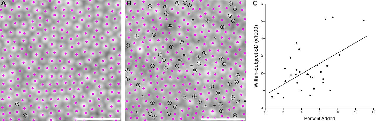
Extremes of the interobserver agreement. Panel A shows the image with the highest agreement with cone identification across all 10 observers while panel B shows the image with the lowest agreement. Pink dots represent the cones identified by the automated algorithm, and black circles represent cones added manually by one or more of the observers (the number inside the circle indicates the number of observers who added that cone). Asterisks in panel B indicate presumed cones that were “missed” by the automated algorithm and not added by any of the 10 observers (these were identified by JC, who was not one of the original 10 observers). Scale bars=20 μm. Panel C shows the correlation between the average percentage of cones added and the total variance within each subject (p=0.0026; r=0.530, 95% CI 0.210 to 0.748).
As has been reported previously for our algorithm,13 there were differences between the number of cones manually added for each subject and each image within each subject. This reflects, in a sense, the ‘accuracy’ of the initial results obtained with the automated algorithm. Intuitively, in subjects where the percentage of cones added was low (ie, the automated algorithm found almost all of the cones in the image), the uncertainty was relatively low. In contrast, the uncertainty increased as the percentage of cones added increased (figure 2C). In addition, there were occasional cells that appear to be missed by the automated algorithm and all 10 observers (figure 2B, asterisks). Taken together, these data demonstrate the need for more robust automated algorithms for cone detection in images of varying quality.14
Experiment 2: inter-instrument
The inter-instrument study included 20 subjects that were each imaged on 2 instruments at the same 8 parafoveal locations, thus 320 observations were available for data analysis. Figure 3 shows parafoveal montages from the same subject acquired using two different AOSLOs.

Parafoveal montages of subject JC_0832 acquired using two different AOSLOs. This is presented to demonstrate the size of the scanning raster and the relationship between the foveal centre and the approximate sampling locations. The large white box represents the extent of the AOSLO scanning raster (1×1°), with the approximate location of the foveal centre marked with a white circle at the centre of the box. The subject was instructed to fixate at each of the four corners of the scanning square and at the middle of each of the four edges. These imaging locations are marked with the smaller white squares and represent the eight locations where cones were identified by a single observer. The small white squares are 55×55 μm in size, which is the area over which density was computed. Scale bar is 100 μm.
Table 2 shows the ICC and 95% CI for the cone density metrics at each location. The ICC ranged from 0.931 to 0.975, indicating that between 93.1 and 97.5% of the total variability can be attributed to variability between subjects while the remaining 2.5–6.9% is due to differences between the devices.
Inter-instrument summary
Discussion
The ability to image the photoreceptor mosaic in the living human retina offers enormous potential for the study of a variety of retinal diseases. Our data indicate that, in normal eyes, reliable estimates of cone density are attainable from reflectance confocal AOSLO images—across different observers and different instruments. Until now, estimates of the reliability and repeatability of such measures were limited to a few anecdotal/empirical reports.21–24 Though they arrived at fairly similar conclusions, it is important that appropriately powered, prospective studies be used to evaluate different cone identification algorithms and retinal imaging systems as their performance is likely to be variable. In addition, it is important to note that our interobserver study only examined interobserver variability for cone density analysis and did not isolate any effect of the use of different operators to collect the AOSLO data between subjects (though the same operator was used to collect the three image sequences within a given subject). As a result, there may be additional variability due to operator-dependent differences in image acquisition, though we believe these to be negligible in the face of other factors (eg, tear film) that impact image quality between subjects.
The repeatability and reliability of cone density measurements in eyes with retinal disease and older eyes with normal vision remains to be assessed. It is likely that performance will be worse, making it even more critical to conduct similar reliability and repeatability studies in these populations. However, such studies bring with them a number of complications. For example, the appearance of the cone mosaic in these eyes can be quite disrupted, in some cases making it difficult to determine whether a given reflective object is a cone, a rod or some other reflective structure in the retina. Furthermore, images from eyes with retinal degeneration may be of lower quality due to lens or vitreous opacities, epiretinal membranes, cystoid macular oedema, high refractive error and tear film abnormalities.21 Images from older eyes may also be of lower quality due to small pupil diameters, lens opacities, epiretinal membranes and tear film abnormalities. Thus, output from any automated algorithm would likely need more input and modification from a trained observer in eyes with retinal degeneration. In addition, most conditions are progressive, meaning that intersession studies need to be carefully monitored to avoid confounding progression with poor repeatability of the algorithm. Finally, it is possible that performance will vary across different diseases, perhaps as a function of the pattern of cone degeneration. For example, patients with albinism or inherited colour vision deficiencies can have significantly disrupted cone mosaics, but the conditions are likely static and current imaging data reveal high-contrast cone structure in these patients.6 ,25 ,26 In contrast, retinitis pigmentosa and choroideremia have non-uniform cone loss across the retina,5 ,8 ,9 resulting in ‘transition zones’ in which cone structure transitions from normal near the central retina to disrupted in the perifoveal/peripheral retina. In these eyes, the performance of any manual or automated algorithm may even vary as a function of retinal location.
This study has demonstrated high reliability of cone density measurements made across different observers and different instruments. An intriguing idea to promote future studies would be the creation of an open-access image repository, to which different groups could contribute images from different systems (commercial- or research-grade), of varying quality, and from different eyes and retinal locations. Providing labs that have expertise in the development of image analysis algorithms with access to a rich database of images should result in more robust and widely applicable tools, as opposed to ‘black-box’ approaches that work for only one lab or one device.
References
Footnotes
-
Contributors Designed the study: BSL, ST, AP and JC. Collected data: BSL, AP, RFC, LL, MW, PG, VM, YNS, NS, GY, AKG, MEP, BJL, JLD and JC. Analysed data: BSL, ST, AV, AP, RFC, AD and JC. Drafted manuscript: BSL and JC. Edited manuscript: BSL, MEP, BJL, AD, JLD and JC. Approved final manuscript: BSL, ST, AV, AP, RFC, LL, MW, PG, VM, YNS, NS, GY, AKG, MEP, BJL, AD, JLD and JC. Obtained funding: MEP, AD, JLD and JC.
-
Funding This study was supported by NEI grants P30EY002162 (UCSF), P30EY001931 (MCW), R01EY017607 (JC), T32EY014537 (MAW) and K08EY021186 (MEP). Additional support from unrestricted departmental grants from Research to Prevent Blindness (Medical College of Wisconsin, UC San Francisco, Casey Eye Institute), a Clinical Center Grant from the Foundation Fighting Blindness (JLD), an Individual Investigator Grant from the Foundation Fighting Blindness (JC), a Career Development Award from the Foundation Fighting Blindness (MEP), the Thomas M. Aaberg, Sr., Retina Research Fund (MCW), That Man May See, Inc. (JLD), The Bernard A. Newcomb Macular Degeneration Fund (JLD), Fight for Sight Summer Student Fellowship (AKG) and Hope for Vision (JLD). This publication was conducted in part in a facility constructed with support from Research Facilities Improvement Program Grant Number C06RR016511 from the National Center for Research Resources, National Institutes of Health. AD-S is the recipient of a Career Development Award from Research to Prevent Blindness and a Career Award at the Scientific Interface from the Burroughs Wellcome Fund. This project was supported in part by the National Center for Advancing Translational Sciences, National Institutes of Health, through grant number UL1TR000055. Its contents are solely the responsibility of the authors and do not necessarily represent the official views of the NIH.
-
Competing interests None.
-
Ethics approval Medical College of Wisconsin Institutional Review Board.
-
Provenance and peer review Not commissioned; externally peer reviewed.