Article Text

Abstract
Aims To describe two approaches for improving the detection of glaucomatous damage seen with optical coherence tomography (OCT).
Methods The two approaches described were: one, a visual analysis of the high-quality OCT circle scans and two, a comparison of local visual field sensitivity loss to local OCT retinal ganglion cell plus inner plexiform (RGC+) and retinal nerve fibre layer (RNFL) thinning. OCT images were obtained from glaucoma patients and suspects using a spectral domain OCT machine and commercially available scanning protocols. A high-quality peripapillary circle scan (average of 50), a three-dimensional (3D) scan of the optic disc, and a 3D scan of the macula were obtained. RGC+ and RNFL thickness and probability plots were generated from the 3D scans.
Results A close visual analysis of a high-quality circle scan can help avoid both false positive and false negative errors. Similarly, to avoid these errors, the location of abnormal visual field points should be compared to regions of abnormal RGC+ and RNFL thickness.
Conclusions To improve the sensitivity and specificity of OCT imaging, high-quality images should be visually scrutinised and topographical information from visual fields and OCT scans combined.
- Glaucoma
- Imaging
- Optic Nerve
- Psychophysics
This is an Open Access article distributed in accordance with the Creative Commons Attribution Non Commercial (CC BY-NC 3.0) license, which permits others to distribute, remix, adapt, build upon this work non-commercially, and license their derivative works on different terms, provided the original work is properly cited and the use is non-commercial. See: http://creativecommons.org/licenses/by-nc/3.0/
Statistics from Altmetric.com
Introduction
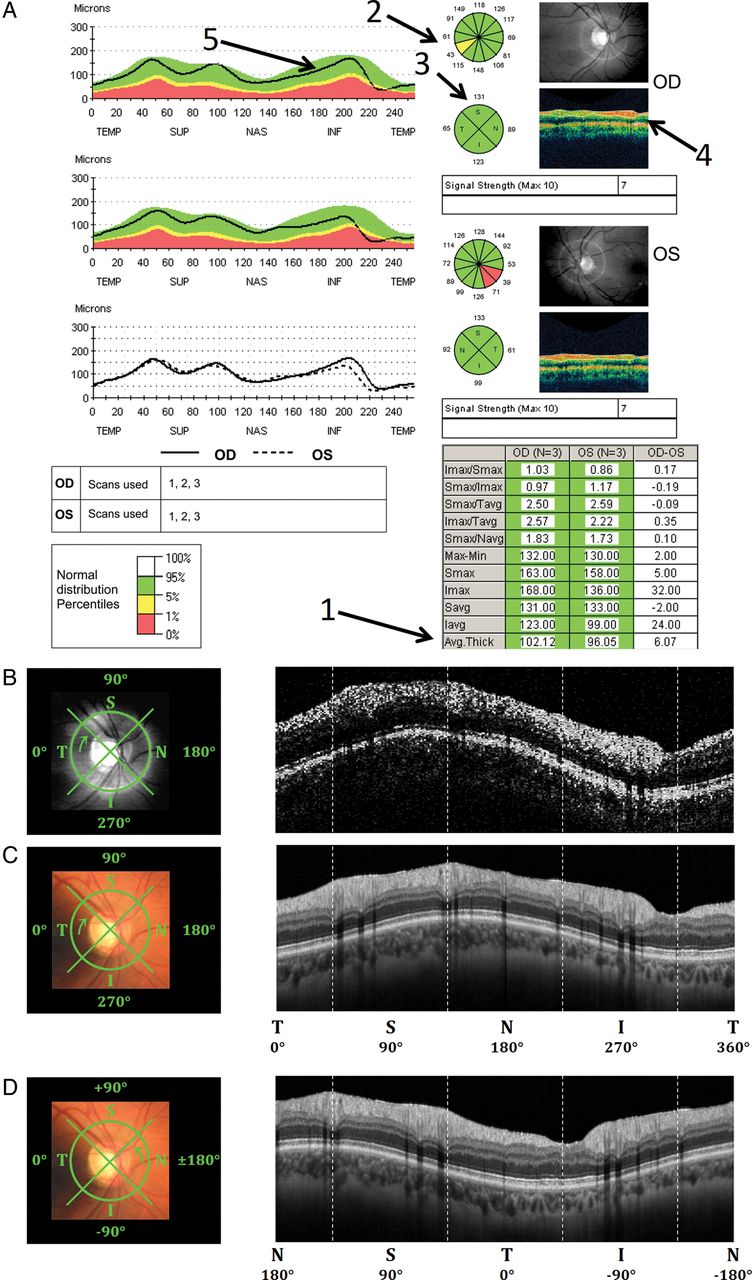
At one time, there was only one commercially available optical coherence tomography (OCT) machine and glaucoma specialists depended upon the summary report (figure 1A) based upon the most commonly used protocol. Numerous studies using this time-domain (td) OCT machine found that the average retinal nerve fibre layer (RNFL) thickness (arrow 1), clock hour thickness (2), and quadrant thickness (3) provide good sensitivity and specificity for detecting glaucomatous damage (see references1–4 for reviews). These RNFL thickness measures were obtained separately from three scans and averaged for this report; the machine was too slow to average multiple images within a scan protocol. One of these scans is shown in figure 1A (4) and the raw data for this same scan is enlarged and presented in grey scale in figure 1B. Given the relatively poor resolution of this peripapillary image, the success of this report is a testimonial to the robustness of these derived RNFL measures, as well as to those who developed the technique and this report.5–8

Peripapillary retinal nerve fibre layer data from Patient 1, showing (A) the report from the Zeiss Stratus time-domain optical coherence tomography (tdOCT) machine based on the average of 3 scans for both eyes (RNFL Thickness (3.4) protocol), (B) the TSNIT circle scan path on top of infrared fundus (left) and a single raw circle tdOCT image (right) for the right eye, (C) the sdOCT TSNIT circle scan path on top of fundus (left) and averaged circle sdOCT image (right) for the same eye, and (D) the sdOCT NSTIN circle scan path (left) and averaged circle sdOCT image (right).
With the advent of newer technology, such as the spectral domain (sd) OCT, the quality of the images became substantially better. For example, compare the scan in figure 1B to the sdOCT scan in figure 1C. The improvement in quality was partly due to improved spatial resolution, but was largely due to the averaging of multiple images within a scan (50 in the case of figure 1C) made possible by a substantially faster scan rate. In addition, because of these improvements, so-called three-dimensional (3D) scans (ie, cube or volume scans) of the regions around the disc and macula became possible. In particular, multiple lines scans can be obtained within a single scan protocol. From these images, 2D measures of the retinal ganglion cell (RGC) and RNFL thickness can be derived.
While the sdOCT allows us to see spatial detail not easily seen on the earlier tdOCT scans, our analyses have not kept pace in at least two ways. First, one of the advantages of sdOCT is that it provides topographical information about RGC and RNFL abnormalities. Thus, local RGC and RNFL loss can be topographically compared to local loss in visual field (VF) sensitivity,9 ,10 as patients are routinely tested with static automated perimetry (SAP). This should improve sensitivity and specificity for detecting glaucomatous damage as SAP measurement errors should be largely independent of OCT measurement errors. Second, the improved sdOCT images allow for a direct visual analysis of the scans, much the way MRI scans are analysed, rather than depending entirely upon computer-driven summary statistics.
The purpose here is to describe two approaches for improving the detection of glaucomatous damage; one approach combines a topographical comparison of OCT and VFs and a second involves a qualitative analysis of OCT scans. These approaches are illustrated below in a one-page report.
Methods
The data from five eyes of five patients, were used to illustrate our approach. All five had glaucomatous optic neuropathy on stereophotography evaluation and all were part of previously published studies.11 ,12 They had 24-2 and 10-2 VFs tests obtained with the SITA-standard protocol (Humphrey VF Analyzer; Carl Zeiss Meditec, Dublin, California, USA); for inclusion, the mean deviation (MD) on the 24-2 VF had to be better than −6 dB.12 Written informed consent was obtained from all of the participants. Procedures followed the tenets of the Declaration of Helsinki, and the protocol was approved by the institutional review board of Columbia University.
OCT protocol
A sdOCT machine (3D OCT-2000, Topcon) and the following three scan protocols were used: 6.0×6.0 mm 3D disc (512 A-scans by 128 B-scans); 6.0×6.0 mm 3D macula (512 A-scans by 128 B-scans); and 3.4 mm dia. circle (average of 50 scans; 1024 A-scans). The circle protocol involved averaging 50 individual scans and thus produced an image of relatively high-quality. (Note that shadowgrams (see inset in panel E of figures 3 (green arrow), 5 and 6) can be examined for artefacts such as excessive eye movements, blinks, etc.)

Visual field (VF) and spectral domain optical coherence tomography (sdOCT) data for Patient 2 along with models relating VF locations to OCT, all shown as if for right eye. (A) The NSTIN averaged circle sdOCT image with computer-derived retinal nerve fibre layer (RNFL) segmentation (green lines) and corresponding circle scan path on top of fundus (inset). (B) The averaged circle RNFL thickness (grey dashed line) calculated based on the segmentation in (A) and the extracted circle RNFL thickness (solid black line), with regions corresponding to the superior (magenta) and inferior (dark blue) macula in unique colours. Both RNFL thickness plots are superimposed on coloured regions indicating the 95% to 5% (green), 5% to 1% (yellow), and less than 1% (red) ranges of normative data. The red vertical lines indicate the average location of the major blood vessels in a group of patients. (C) The 24-2 VF for the same patient with (D) a model relating the locations of the VF to regions of the circle scans. (E) The 10-2 VF for the same patient with (F) a model relating the locations of the VF to regions of the circle scans. The bold dark blue line indicates the macular vulnerability zone (MVZ).
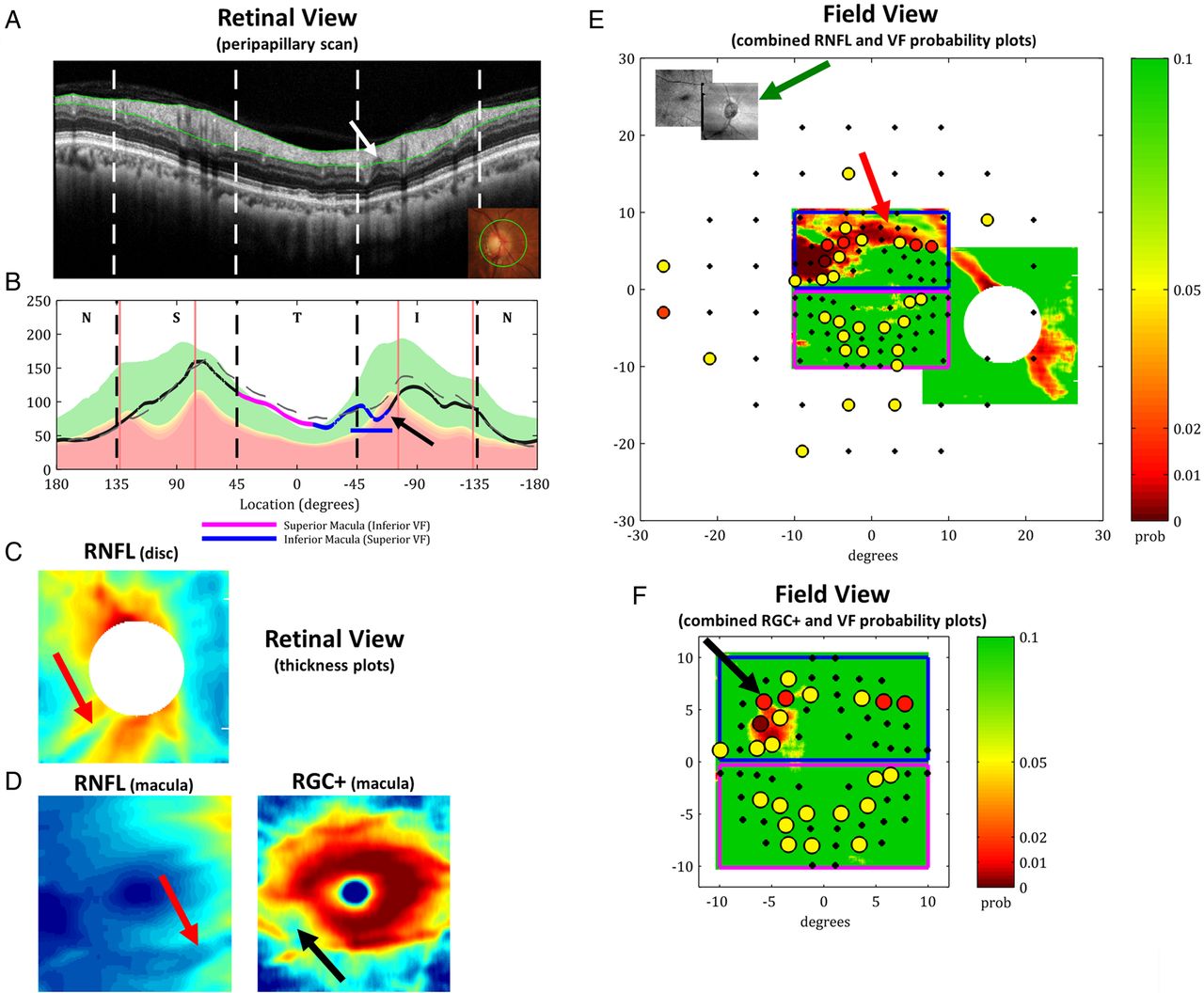
The single-page spectral domain optical coherence tomography report for Patient 3 showing (A) an enlarged averaged circle scan in NSTIN view as in figure 2A, (B) the corresponding retinal nerve fibre layer (RNFL) thickness as in figure 2B, (C) the 2D RNFL thickness from the 3D disc scan, (D) the 2D RNFL (left) and retinal ganglion cell (RGC)+ (right) thicknesses from the 3D macular scan, (E) the co-registered macular and disc 2D RNFL thickness probability plots in field view with the 24-2 and 10-2 visual field (VF) test point probabilities superimposed (see colour bar) with an inset of the co-registered shadowgrams of the 3D scans (green arrow), and (F) the macular 2D RGC+ thickness probability plot in field view with the 10-2 VF test point probabilities superimposed (see colour bar) as in (E).

(A) The 24-2 and (B) 10-2 visual field (VF) data for Patient 3. (C) The 10-2 VF data for Patient 4, (D) the 24-2 VF data from 2013 for Patient 5, and (E) enlargements of a hole observed in the averaged circle scan of Patient 5 in both 2013 (left) and 2010 (right).

The single-page spectral domain optical coherence tomography report for Patient 4 as in figure 3 showing diffuse retinal ganglion cell (RGC)+ thinning (panel D, right). The agreement of the RGC+ (panel F) and retinal nerve fibre layer (RNFL) (panel E) probability plots with the visual field (VF) probability plot suggests diffuse macular damage.
OCT analysis
Peripapillary RNFL analysis
The high-quality peripapillary image produced by the circle scan was qualitatively analysed as described in the Results. In addition, this image was segmented by the machine's software and a RNFL thickness plot produced. While the circle scan has the advantage of being of high quality, it can be off-centre if the patient has considerable trouble fixating or the operator is not careful. The fundus photo with the superimposed scan location (inset in panel A of figures 2, 3, 5 and 6) provides some information about how well centred the scan was.
The commercial software also derives a peripapillary RNFL thickness plot from the segmentation of the 3D disc scan, by centring a circle after the scan is obtained. To distinguish this plot from the one based upon the high-quality averaged circle scan, it will be called the ‘extracted circle RNFL plot’. (Note: As technological advances improve the quality of the 3D scan, the circle scan can be replaced by an image of the peripapillary circle extracted from the 3D scan.)
3D RNFL and RGC+ thickness maps
As previously described,9 RGC+ and RNFL thickness maps were derived from the macular and disc 3D scans and turned into probability plots by comparing the thicknesses to normative values.
Results
Below we describe elements of a report for detecting RGC/RNFL damage based upon sdOCT imaging. The report is designed to illustrate the power of combining VF and OCT information, as well as the value-added in carefully examining the OCT images.
Reports should display RNFL thickness plots as NSTIN, not TSNIT plots
In the original tdOCT report, the peripapillary circle scan (arrow 4 in figure 1A) was presented with the nasal quadrant (N) in the middle and the temporal (T) quadrant divided between the left and right ends. The accompanying RNFL thickness plot (arrow 5 in figure 1A) has been called the ‘TSNIT plot’. Instead, we recommend using a ‘NSTIN plot’, in which the most important portion of the disc for visual function, the temporal quadrant, is in the middle (figure 1D). As illustrated below, this allows for easier visualisation of the relationship between RNFL thinning and VF defects.
Reports should contain an enlarged image of the circle scan
Figure 2A shows the averaged circle scan from Patient 2 with the computer-derived borders of the RNFL in green. There are two reasons for including an image larger than seen in the tdOCT report in figure 1A (arrow 4). First, the validity of the computer-marked borders can be assessed. All current OCT computer algorithms make mistakes (segmentation errors), which will be typically overlooked if the scan image is presented as a small inset as in figure 1A. Epiretinal membranes, vitreous detachments, and poor image contrast can lead to segmentation errors and thus errors in the associated RNFL thickness measures. The enlarged, averaged circle scan has sufficient detail so that these errors can be identified.
Second, the high-quality image allows for a qualitative assessment of the details of the scan. For example, in figure 2A local RNFL thinning can be seen in two regions (see white arrows). Other details of interest can be seen in some circle scans as illustrated below.
Look for regions of abnormal thinning on the RNFL plot and compare to scan
After scrutinising the averaged circle scan image, the RNFL thickness plots should be examined. The dashed and solid curves in figure 2B are the RNFL thickness plots from the averaged circle and 3D scans, respectively. If these curves agree and the segmentation seen on the scan appears accurate, these plots can be trusted. If they disagree, it is usually possible to decide why.
For example, the averaged circle (dashed) and extracted circle (solid) RNFL thickness plots from Patient 3 in figure 3B disagree in two locations. First, the thickness in the temporal quadrant and part of the superior quadrant is slightly greater in the case of the averaged circle, probably because the circle scan is off-centre; see the fundus photograph (inset in panel A). Second, and more important, there is a suggestion of a small local defect on the extracted circle RNFL plot (solid), but not on the averaged circle plot (dashed). A close examination of the scan in panel A, indicates a small, local thinning, which the algorithm appears to underestimate on the averaged circle scan. This is discussed further below.
After assessing the veracity of the RNFL plot (figure 2B), the regions of abnormal thinning can be identified. In this case, the RNFL plot falls well below the 99% confidence limit in the same regions (black arrows in figure 2B) that show local thinning on the scan in figure 2A (white arrows).
Examine the general topographical agreement between peripapillary RNFL thinning and loss in VF sensitivity
With a little practice, the topographical agreement between peripapillary RNFL thinning and VF defects can be assessed qualitatively. To make this assessment, one needs to take into consideration the relationship between regions of the disc and regions of the VF.
Figure 2 illustrates this relationship. The 24-2 pattern deviation (PSD) plot for this eye is shown in panel C. The red and light blue arrows in panel B mark the temporal half of the circle scan, that is, they extend from +90° to −90° as shown in panel D. The corresponding region of the 24-2 VF is enclosed within the light blue and red contours in panel C. These contours were drawn to be in general agreement with previous work.13 ,14 While these contours are approximate, and will differ somewhat among individuals,13 ,15 they are useful for deciding whether there is agreement among the OCT and VF findings.
The dashed red and blue horizontal lines along the x-axis in figure 2B show the regions of the RNFL plot that correspond to the abnormal regions of the VF (ie, the points falling within the dashed ellipses in C). In this case there is excellent agreement.
The RNFL plot also suggests there is damage in the macula, defined here as the central ±8°. To facilitate the detection of macular damage on the RNFL plots, the regions of the scan associated with the RGC fibres from the central ±8° retina are coded as magenta (superior retina/lower VF) and dark blue (inferior retina/upper VF). These boundaries (see panel F), as well as the corresponding regions on the 10-2 (panel E), are based upon a recent map of the macula.16 Note that macular damage is confirmed by the 10-2 VF in panel E.
Look for macular damage especially in the macular vulnerability zone
We have identified two types of macular damage on OCT scans.12 One type, considered below, is diffuse/widespread and is typically relatively shallow and difficult to identify with RNFL scans. The second tends to be deeper and to occur in a relatively narrow portion of the inferior disc labelled macular vulnerability zone (MVZ) in figure 2F.
This local macular damage easily can be missed if one does not look closely at the high-quality averaged circle scan and the RNFL plots. Figure 3A,B shows what appears to be a relatively normal RNFL thickness plot, although there is probably local nasal thinning far outside the 24-2 VF. The commercial report (not shown) indicated normal RNFL thickness in the inferior, temporal and superior quadrants and the associated clock hours. The 24-2 VF (figure 4A) appeared normal as well with a MD of −1.50 dB, a PSD of 1.16 dB, and a glaucoma hemifield test (GHT) within normal limits. However, as mentioned above, the extracted circle RNFL plot from the 3D scan (solid curve in figure 3B) shows a very local abnormal region (arrow). Given the VF results, this local abnormality could easily be overlooked. In any case, the scan in figure 3A shows a small local thinning (white arrow). This local thinning is in the middle of the MVZ, which is shown as the horizontal dark blue line. The damage in the MVZ can be missed on 24-2 VF tests because they poorly sample the region of glaucomatous damage of the macula seen on OCT.16
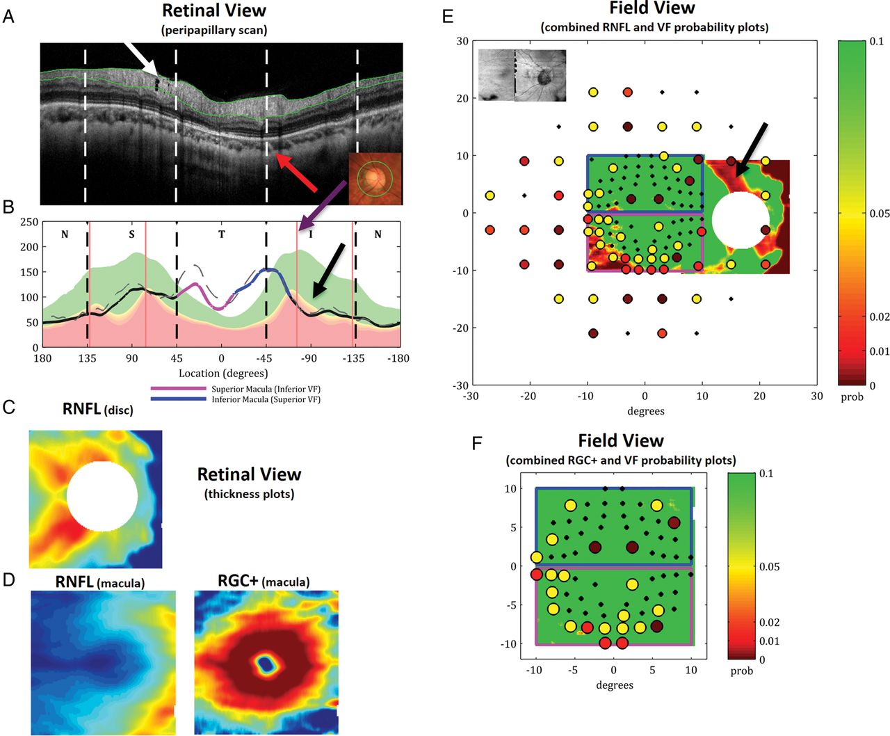
The single-page spectral domain optical coherence tomography report for Patient 5 as in figure 3 illustrating the need for a close scrutiny of peripapillary scans (panel A). The peripapillary retinal nerve fibre layer (RNFL) thickness plot (panel B) and the RNFL probability plot (panel E) suggest an abnormally thin RNFL associated with the upper visual field. However, this is probably a false positive, as indicated by a close examination of the location of the inferior temporal blood vessels (red arrow in panel A) in this eye to the average location in a group of patients (purple arrow in panel B), as well as the abnormally thick RNFL in the temporal quadrant. The repeat visual fields (VFs) are consistent with this interpretation. On the other hand, the presence of a hole (black arrow in panel A) suggests that there may be very early glaucomatous damage in the superior disc.
The patient's 10-2 VF (figure 4B) shows a subtle defect in the general region one would expect from the model of macular damage.16 However, given the subtle nature of both the OCT and VF changes, there is reason for scepticism. Figure 3 is our one page report of RGC/RNFL damage; the other panels, described below, confirm the damage is real.
Examine the RGC layer thickness maps obtained from the macular 3D scan
RGC thickness maps are useful for identifying macular damage, which can be missed on peripapillary RNFL analysis. In general, the commercial machines supply an analysis of macular 3D scans that includes RGC thickness. In some cases, this is the thickness of the combined RGC, inner plexiform layer (IPL) and RNFL, while in others it is the thickness of the combined RGC+IPL (called here RGC+). Figure 3D (right panel) shows the patient's RGC+ thickness derived from the macular 3D scan and displayed in pseudo-colour. By comparing the local thickness values to healthy controls, a probability plot can be created as shown in figure 3F. This probability plot is displayed in field view. The abnormally thin RGC+ layer (black arrows in figure 3D,F) argues for macular damage in this eye.
Examine the RNFL layer thickness maps obtained from macular and disc 3D scans
From the 3D scans of the disc most commercial machines produce RNFL thickness plots as shown in figure 3C. A RNFL thickness plot can also be produced for the macular 3D scans as shown in figure 3D (left). By comparing the thickness values to healthy controls, this thickness plot can be turned into a probability plot. For the report, the RNFL probability plots from the macular and disc 3D scans are combined by aligning the blood vessels and then displayed in field view (figure 3E). The local macular damage is clearly apparent in this RNFL thickness analysis as indicated by the red arrows in panels C, D (left) and E.
Examine the topographical agreement between local RNFL and RGC+ thinning and local loss in VF sensitivity
The best way to assess the topographical agreement between RNFL thinning and VF sensitivity loss is to superimpose the probability plots for each as previously described.9 This analysis is shown on the right side of our report.
Figure 3F shows the points from this patient's 10-2 VF (figure 4B) superimposed on the field view of the RGC+ probability plot. The significance levels of the 10-2 points and RGC+ thickness are colour-coded using the same continuous probability scale. To make this comparison, the locations of the VF points need to be adjusted to account for the displacement of the RGCs in the fovea.9 ,10
In a similar manner, in figure 3E the points of the 24-2 and 10-2 VF are superimposed upon the RNFL probability plot (field view) and coded with the same continuous probability scale. There is good local agreement between the OCT and VF results for the upper VF/inferior retina.
While it may be difficult for manufacturers to incorporate VF data into their software, it should be relatively easy for them to indicate the 24-2 and 10-2 locations on the OCT probability plots and leave it to the clinician to circle the VF points that are abnormal.
Using the report to detect diffuse macular damage
The report for Patient 4 in figure 5 illustrates an example of what we believe is diffuse macular damage.12 This patient's 10-2 VF (figure 4C) had a MD of −4.15 dB (p<1%) and the total deviation values showed a relatively homogeneous loss across the VF. Given that the PSD was normal, many would attribute this diffuse loss of sensitivity to non-glaucomatous factors. The peripapillary RNFL plot in figure 5B is also ambiguous with the region corresponding to the macula (magenta and dark blue) falling in the normal (green) or borderline (yellow) region. The comparison of RGC+ and VF abnormalities in panel F, however, suggests diffuse macular damage. The RNFL and VF comparison in panel E agrees. On exam, this patient did not have cataracts, but did have a best corrected visual acuity (BCVA) of 20/50, also consistent with diffuse damage.
Carefully examine the actual scan images
There is much to be learned by carefully examining the actual OCT scan images. Below, we illustrate three examples.
False positives and the location of blood vessels
Figure 6 shows our report for the right eye of Patient 5. A glaucoma specialist noted peripapillary atrophy and diffuse thinning on fundus stereo photograph. The report from the commercial machine showed abnormal RNFL thinning in the inferior quadrant. Our report appeared to confirm this finding (black arrows in figure 6B). However, while the OCT analysis was consistent with local damage, the fundus exam and VF (figure 4D) were consistent with diffuse damage. On closer analysis, we concluded that the OCT result was a false positive, an example of what has been called ‘red disease’.17 Notice the abnormally thick RNFL in the temporal quadrant in figure 6A,B. The major blood vessels (BVs) in this eye are located more temporally than the average location for the controls. The red lines in panel B show the average locations of the major four groups of BVs for a group of patients.18 The red arrow in panel A indicates the location of the inferior-temporal (IT) BVs in this eye, while the purple arrow shows the average location of the IT BVs. As expected, the location of the IT BVs correspond to the location of the inferior peak of the RNFL plot (peak of green in panel A) in healthy controls.19 This is, in part, due to the direct contribution of the BVs to the RNFL thickness and in part due to the fact that the thickest region of RNFL tends to be close to the major BVs.19 In any case, the location of the IT BVs in this eye is probably the reason for the abnormally thick RNFL in the temporal quadrant and the abnormally thin RNFL in the inferior quadrant. The 24-2 VF is probably a false positive as well. Note that the 24-2 test from 2012, 1 year earlier, was normal, while the 24-2 VF obtained 2 years earlier showed diffuse loss.
Hypodense (holes)
While the inferior quadrant of the RNFL profile of this eye illustrates a false positive OCT result, the scan in figure 6A has evidence of local damage in the superior quadrant of the disc. In particular, there is a hypodense region (white arrow in figure 6A). We have shown that these holes are actually tunnels that follow an arcuate pattern and are almost surely very local, and very small, RNF bundle defects.20 We have only seen them in patients with glaucoma or patients who are glaucoma suspects.21 They also show progression as seen for this eye in figure 4E.
Examine horizontal and vertical macular scans for outer retinal damage
Finally, we routinely examine the 3D macular scans, as well as a high-quality horizontal line scans through the macula, for signs of outer retinal damage. This is particularly important in eyes with reduced visual acuity. It is common to see previously unnoticed signs of epiretinal membranes, age-related macular degeneration, oedema, and macular holes in glaucoma patients and suspects.22
Discussion
While once there was a single OCT report used to identify glaucomatous damage, now every commercial machine offers more than one glaucoma report. However, by and large, these reports fail to take full advantage of the spatial detail available. We argued above that the effectiveness of the OCT could be improved by a qualitative analysis of enlarged, high-quality images and by a topographical comparison of the abnormal regions seen on OCT to those seen on VFs. Our one-page report was developed to incorporate this information.
However, no one report will suffice. The high-quality OCT scans have all the complexities of MRI scans, as well as better spatial resolution. Yet, MRI scans are not analysed by computer algorithms and summarised in simple summary statistics and diagrams, as is typically the case with OCT scans. In fact, relying solely on summary statistics plays a major role in apparent disagreements between the results of VF and OCT tests.23 In the case of MRI scans, radiologists read and interpret the scans for other specialists, while in the case of OCT scans, ophthalmologists are left to interpret the scans on their own.
While the report developed here is meant to help ophthalmologists in this interpretation, it will not suffice. On one hand, the summary statistics and diagrams seen in figure 1A are still of use and new summary statistics combining VF and OCT information are being developed.24–30 The sensitivity and specificity of these various summary statistics need to be compared to alternative analyses, such as the report describe here with and without summary statistics. On the other hand, the full power of the OCT will rely on a careful analysis of high-quality images performed by individuals trained to read these scans, much the way a radiologist reads an MRI. This will be increasingly the case as OCT image quality continues to improve. Admittedly, for many cases a simple report or summary statistic may do. However, for difficult and ambiguous cases, the non-specialist may need to rely on a member of their department/group who has considerable experience analysing OCT scans.
Acknowledgments
We thank Paula Alhadeff, Dana Blumberg, and Jeffrey Liebmann for their comments and advice, and especially Drs Robert Ritch, Jeffrey Odel and Gustavo de Moraes for their help and support throughout this project.
References
Footnotes
-
Contributors Both authors were responsible for the design of the study and interpretation of the data, as well as preparation, review and approval of the article.
-
Funding The study was supported by National Institutes of Health Grant R01-EY-02115 and a grant from Topcon, Inc.
-
Competing interests The study was supported by a grant from Topcon, Inc.
-
Patient consent Obtained.
-
Ethics approval The Institutional Review Board of Columbia University.
-
Provenance and peer review Commissioned; externally peer reviewed.