Loss of information and statistical power

Dichotomisation results, first, in the loss of descriptive information on the study population. For example, the nature and extent of differences between individuals with low vision is lost when visual acuity is dichotomised as having/not having low vision. Second, with dichotomisation there is loss of information on between-subject variability in the study population as, for instance, subjects with similar outcome measures but on either side of the threshold will be described and analysed as different while two subjects with values that are on the same side of the threshold, but one near and another a long way from the threshold, will be treated as if they are the same. In addition, it is not possible to quantify linear relationships after dichotomising a variable (eg, it is not possible to quantify the change in mm Hg of IOP per mm Hg of systolic blood pressure (SBP) increase if IOP has been dichotomised), and any non-linear relationship would be masked by dichotomisation.

There may also be a loss of statistical power (the probability of detecting a true effect of a particular size should it exist) associated with dichotomisation. To maintain statistical power equivalent to that for continuous data, dichotomised data require an increase in sample size. Table 1 shows the sample size required to detect a significant association (correlation) between IOP and SBP, at the 5% significance level, assuming a linear change of 0.035 mm Hg in IOP per mm Hg of SBP4 ,5 under two scenarios: (a) IOP as a continuous variable (sample size denoted as n_o) and (b) IOP dichotomised using three different cutpoints (ie, different values for the threshold of IOP that defines the two IOP categories; sample size denoted as n_d). Sample size values were calculated using the sample size formulae available for the correlation coefficient6 for scenario (a), and for the two-sample t test7 (Equation 5.2) for scenario (b). Simulations were generated to calculate n_d and the reduction in power for scenario (b) shown in table 1.

When IOP is dichotomised, a larger sample size (n_d) is needed to detect a significant association while maintaining the same power as an analysis with sample size n_o using IOP as a continuous variable. For example, when IOP is analysed as continuous, the sample size required is 119 individuals for a power of 90%. If IOP is dichotomised using the mean as the cutpoint (14.5 mm Hg), then the sample size required to maintain 90% power increases to 175 individuals—56 additional patients. If the condition of interest is rare, this increase in the required number of patients might render a study infeasible. Alternatively, a reduction in power of at least 15% would occur if the sample size remains at n_o=119 and IOP was dichotomised.

Introduction of bias in associations

In clinical research, the association observed between a risk factor and an outcome can be affected by background factors (such as age) that are associated with the risk factor while also having an influence on the outcome. These background factors are known as confounders. If confounders are present, the estimation of the association of interest between the risk factor and outcome can be biased. Clinical trials are designed to minimise the effect of confounding, with subjects being randomised to intervention or control groups to ensure the groups are balanced with regard to the background factors. However, in epidemiological and other clinical studies, estimates may be biased if the effect of the confounding variable is not properly accounted for in the analysis. If a confounder is taken into account but is dichotomised, this may remove some but not all of the effects of confounding and hence still result in bias.8 The magnitude of the bias will depend on the selected cutpoint of dichotomisation and the strength of the confounding effect.

For example, let us investigate if IOP is affected by whether an individual has diabetes. The existing evidence suggests that SBP is related to IOP and also diabetes and as such is a potential confounding variable for the relationship between IOP and whether or not a patient has diabetes (figure 1).

• Download figure
• Open in new tab
• Download powerpoint

Figure 1

Systolic blood pressure (SBP) as a potential confounder of the relationship between diabetes and intraocular pressure (IOP).

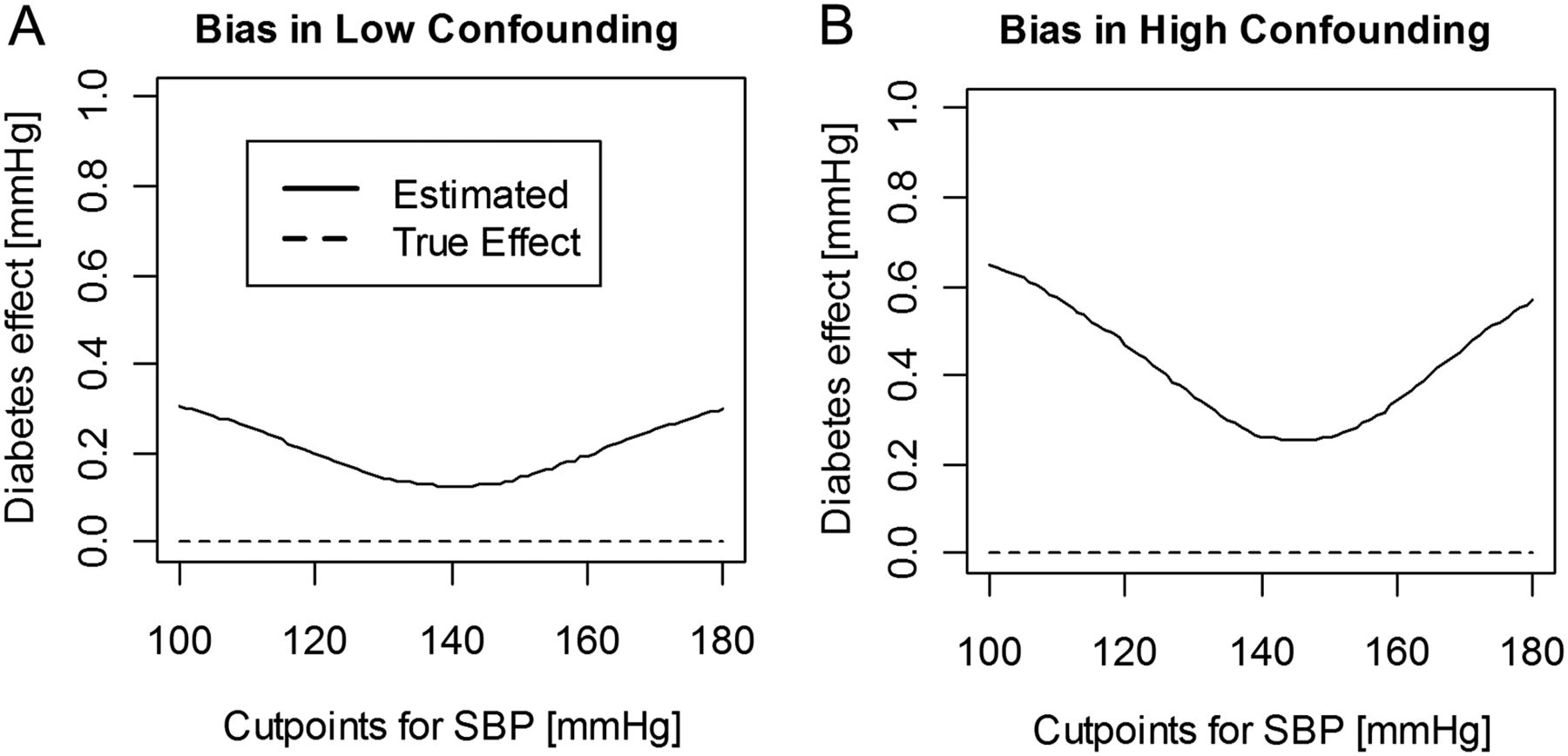
We can fit a linear regression model to estimate IOP with SBP as a continuous covariate and diabetes as a factor with two levels (Yes/No). Let us assume that the true model shows no relationship between IOP and diabetes (ie, a model coefficient of zero for the factor diabetes). The effect of diabetes is correctly estimated as zero using linear regression with SBP as a continuous variable (see dashed lines in figure 2). However, if instead we dichotomise SBP, we find an effect of diabetes on IOP because patients with diabetes are more likely to have SBP above the cutpoint and vice versa (see solid lines in figure 2). In this example, when SBP is dichotomised, data can be fitted using analysis of variance with two factors, diabetes and dichotomised SBP. Figure 2 demonstrates the effect of diabetes adjusted for low and high level of confounding (panels A and B, respectively) dichotomising SBP with a cutpoint of 140 mm Hg (median). In figure 2A, we would estimate IOP to be on average 0.13 mm Hg higher in the diabetic group compared with the non-diabetic group. With a higher level of confounding (figure 2B), that is, a stronger relationship between SBP and diabetes or larger differences between mean SBP in the diabetes and non-diabetes groups, the bias is even higher (0.26 mm Hg). The stronger the confounding between a risk factor and a background variable, the larger the bias introduced by dichotomising the confounding variable. With cutpoint values more extreme than the median, the bias and the probability of concluding that there is a significant effect of diabetes on IOP when there is no true effect (ie, a type 1 error) increase.

• Download figure
• Open in new tab
• Download powerpoint

Figure 2

Biased estimates of the effect of diabetes on intraocular pressure (IOP) when confounder systolic blood pressure (SBP) is dichotomised. This simulation assumes that IOP follows a normal distribution and increases on average by 0.035 mm Hg per 1 mm Hg increase in SBP. We also assume that SBP follows a normal distribution with means of 135 and 145 mm Hg for the non-diabetic and diabetic groups, respectively (A) and 135 and 155 mm Hg for the non-diabetic and diabetic groups, respectively (B). Finally, we assume that mean IOP is the same in those with and without diabetes. The estimated effect of diabetes on IOP is erroneously positively biased if SBP is dichotomised (see solid curves). To illustrate the average bias, this simulation is based on large number of individuals: 50 000 diabetic and 50 000 non-diabetic.

Points for consideration

It is not good practice to power a study, obtain data from a number of individuals and then after completing data collection to underpower the analysis by dichotomisation, thus discarding a substantial amount of the data and information.8 It may be appropriate to dichotomise data in certain cases, when the underlying distribution of the variable shows a clear grouping; however, all decisions regarding cutpoints for categorisation should be prespecified before conducting the analysis and reasons for such decisions stated when writing a paper. It is poor practice, for example, to perform the analysis using various data-derived cutpoints and then select the threshold with the most ‘significant’ result (minimal p value approach). Using a threshold for dichotomisation that is dependent on the study sample and not the population (eg, when the cutpoint is defined as the sample mean or sample median) will result in a different cutpoint for each study. Thus, results of individual studies will not be generalisable and comparisons between studies may be problematic.

In summary, researchers and clinicians need to be aware of and consider the potential loss of information, decrease in statistical power and the bias that may be introduced by dichotomisation of continuous data.