Article Text

Abstract
AIM To recognise automatically the main components of the fundus on digital colour images.
METHODS The main features of a fundus retinal image were defined as the optic disc, fovea, and blood vessels. Methods are described for their automatic recognition and location. 112 retinal images were preprocessed via adaptive, local, contrast enhancement. The optic discs were located by identifying the area with the highest variation in intensity of adjacent pixels. Blood vessels were identified by means of a multilayer perceptron neural net, for which the inputs were derived from a principal component analysis (PCA) of the image and edge detection of the first component of PCA. The foveas were identified using matching correlation together with characteristics typical of a fovea—for example, darkest area in the neighbourhood of the optic disc. The main components of the image were identified by an experienced ophthalmologist for comparison with computerised methods.
RESULTS The sensitivity and specificity of the recognition of each retinal main component was as follows: 99.1% and 99.1% for the optic disc; 83.3% and 91.0% for blood vessels; 80.4% and 99.1% for the fovea.
CONCLUSIONS In this study the optic disc, blood vessels, and fovea were accurately detected. The identification of the normal components of the retinal image will aid the future detection of diseases in these regions. In diabetic retinopathy, for example, an image could be analysed for retinopathy with reference to sight threatening complications such as disc neovascularisation, vascular changes, or foveal exudation.
- image analysis
- image recognition
- neural network
- diabetic diagnosis
- retinopathy
Statistics from Altmetric.com
The patterns of disease that affect the fundus of the eye are varied and usually require identification by a trained human observer such as a clinical ophthalmologist. The employment of digital fundus imaging in ophthalmology provides us with digitised data that could be exploited for computerised detection of disease. Indeed, many investigators use computerised image analysis of the eye, under the direction of a human observer.1-4 The management of certain diseases would be greatly facilitated if a fully automated method was employed.5 An obvious example is the care of diabetic retinopathy, which requires the screening of large numbers of patients (approximately 30 000 individuals per million total population6 7). Screening of diabetic retinopathy may reduce blindness in these patients by 50% and can provide considerable cost savings to public health systems.8 9 Most methods, however, require identification of retinopathy by expensive, specifically trained personnel.10-13 A wholly automated approach involving fundus image analysis by computer could provide an immediate classification of retinopathy without the need for specialist opinions.
Manual semiquantitative methods of image processing have been employed to provide faster and more accurate observation of the degree of macula oedema in fluorescein images.14 Progress has been made towards the development of a fully automated system to detect microaneurysms in digitised fluorescein angiograms.15 16Fluorescein angiogram images are good for observing some pathologies such as microaneurysms which are indicators of diabetic retinopathy. It is not an ideal method for an automatic screening system since it requires an injection of fluorescein into the body. This disadvantage makes the use of colour fundus images, which do not require an injection of fluorescein, more suitable for automatic screening.
The detection of blood vessels using a method called 2D matched filters has been proposed.17 This method requires the convolution of each image with a filter of size 15 × 15 for at least 12 different kernels in order to search for directional components along distinct orientations. The large size of the convolution kernel entails heavy computational cost. An alternative method to recognise blood vessels was developed by Akita and Kuga.18 This work does not include automatic diagnosis of diseases, because it was performed from the viewpoint of digital image processing and artificial intelligence.
None of the techniques quoted above has been tested on large volumes of retinal images. They were found to fail for large numbers of retinal images, in contrast with the successful performance of a neural network.
Artificial neural networks (NNs) have been employed previously to examine scanned digital images of colour fundus slides.19Using NNs, features of retinopathy such as haemorrhages and exudates were detected. These were used to identify whether retinopathy was present or absent in a screened population but allowed no provision for grading of retinopathy. The images with retinopathy still require a grading by a trained observer. Grading greatly improves the efficiency of the screening service, because only those patients with sight threatening complications are identified for ophthalmological management. This task is more complex than identifying the presence of retinopathy because the computer programme must be able to detect changes such as neovascularisation, cotton wool spots, vascular changes, and perifoveal exudation.20 The first step for achieving this aim is to be able to locate automatically the main regions of the fundus—that is, the optic disc, fovea, and blood vessels. The data from these regions can then be analysed for features of sight threatening disease. Identification of the regions of the fundus may also aid analysis of images for other diseases that affect these areas preferentially—for example, glaucoma and senile macular degeneration.
In this study, a variety of computer image analysis methods, including NNs, were used to analyse images to detect the main regions of the fundus.
Methods
In all, 112 TIF (tagged image format) images of the fundi of patients attending a diabetic screening service were obtained using a Topcon TRC-NW5S non-mydriatic retinal camera. Forty degree images were used.
PREPROCESSING OF COLOUR RETINAL IMAGES
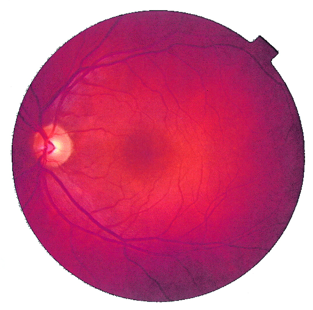
The captured fundus images were of dimensions 570 × 550 pixels. Each pixel contained three values, red, green, and blue, each value being quantised to 256 grey levels. An example can be seen in Figure 1. The contrast of the fundus images tended to diminish as the distance of a pixel from the centre of the image increased. The objective of preprocessing was to reduce this effect and to normalise the mean intensity. The intensities of the three colour bands were transformed to an intensity-hue-saturation representation.21 This allowed the intensity to be processed without affecting the perceived relative colour values of the pixels. The contrast of the intensity was enhanced by a locally adaptive transformation. Consider a subimage,W(i, j), of sizeM×M pixels centred on a pixel located at (i, j). Denote the mean and standard deviation of the intensity within W(i, j)by <f>Wand ςW respectively. Suppose that fmax andfmin were the maximum and minimum intensities of the whole image.

Digital colour retinal image.
The adaptive local contrast enhancement transformation was defined by equations (A1) and (A2) of appendix .
Figure 2 shows the effect of preprocessing on a fundus image, Figure1.

Retinal image after preprocessing by local colour contrast enhancement.
RECOGNITION OF THE OPTIC DISC
The optic disc appeared in the fundus image as a yellowish region. It typically occupied approximately one seventh of the entire image, 80 × 80 pixels. The appearance was characterised by a relatively rapid variation in intensity because the “dark” blood vessels were beside the “bright” nerve fibres. The variance of intensity of adjacent pixels was used for recognition of the optic disc.
Consider a subimage W(i, j) of dimensionsM×M centred on pixel(i, j). Let <f>w(i,j) as defined by equation (A3) be the mean intensity within W(i, j). (IfW(i, j) extended beyond the image, then undefined intensities were set to zero and the normalisation factor was correspondingly reduced.)
A variance image was formed by the transformation
The variance image of Figure 2 is shown in Figure 3 and the location of the optic disc in Figure 7.

The variance image of Figure 2.

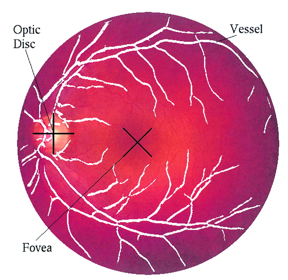
The results of automatic recognition of the main components of the fundus from a digital fundus colour image.
RECOGNITION OF BLOOD VESSELS
Blood vessels appeared as networks of either deep red or orange-red filaments that originated within the optic disc and were of progressively diminishing width. A multilayer perceptron NN was used to classify each pixel of the image.22-24 Preprocessing of the image was necessary before presentation to the input layer of the NN. Pattern classifiers are most effective when acting on linearly separable data in a small number of dimensions. More details are described in appendix .
The values of the three spectral bands of a pixel were strongly correlated. The principal component transformation25 was used to rotate the axes from red-green-blue to three orthogonal axes along the three principal axes of correlation, thus diagonalising the correlation coefficient matrix. The values along the first axis exhibited the maximum correlated variation of the data, containing the main structural features. Uncorrelated noise was concentrated mainly along the third axis while, in general, texture tended to be along the second. The original data were reduced in dimensionality by two thirds by the principal component transformation.
A measure of edge strength was obtained for each pixel by processing the image from the first principal component using a Canny edge operator.26-28 This was used to enhance vessel/non-vessel separability.
NEURAL NETWORK ALGORITHM
Each pixel of a fundus image was classified as vessel or non-vessel. The data input to the NN were the first principal component29 and edge strength values from a subimage of 10 × 10 pixels localised on the pixel being classified, as shown in Figure 4. The net was a three layer perceptron having 200 input nodes, 20 hidden nodes, and two output nodes.
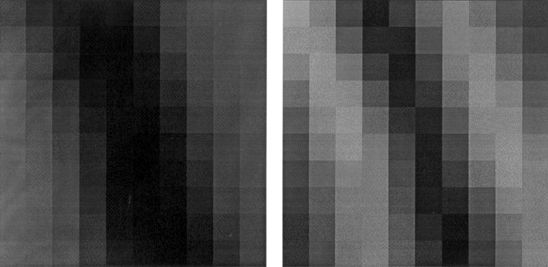
An example of the data input to the net, of size 2 × 10 × 10 pixels. In this example, the pattern was classified as vessel.
A training/validation data set of 25 094 examples, comprising 8718 vessel and 16 376 non-vessel, was formed by hand and checked by a clinician. The back propagation algorithm with early stopping was applied,30
31 using
POST-PROCESSING3233
Figure 5 shows the classification of the entire image into vessel and non-vessel, denoted as black and white respectively.

Classification of the image Figure 2 into vessels/non-vessels.
The performance of the classifier was enhanced by the inclusion of contextual (semantic) conditions. Small isolated regions of pixels that were misclassified as blood vessels were reclassified using the properties that vessels occur within filaments, which form networks. Three criteria were applied—size, compactness, and shape. Regions smaller than 30 pixels were reclassified as non-vessels. The compactness of a region may be expressed using the ratio of the square of the perimeter to the area34—for example, circular discs have a ratio of 4π. Regions whose ratios were less than 40 were reclassified as non-vessels. Approximating a region by an elliptical disc yields a measure of shape in terms of the ratio of the major and minor axes.35 Regions smaller than 100 pixels with a ratio smaller than 0.95 were reclassified as non-vessels as can be seen in appendix . Figure 6 shows the effect of such post-processing on an image.

The classified image after post-processing to remove small regions.
RECOGNITION OF THE FOVEA
The centre of the fovea was usually located at a distance of approximately 2.5 times the diameter of the optic disc, from the centre of the optic disc. It was the darkest area of the fundus image, with approximately the same intensity as the blood vessels. The fovea was first correlated to a template of intensities. The template was chosen to approximate a typical fovea and was defined by
where (i, j) are relative to the centre of the template. A template of size 40 × 40 pixels was employed, the standard deviation of the Gaussian distribution being ς = 22. Given a subimage W(i, j) centred on pixel(i, j) of dimensionsM×M with intensitiesg(k, l), (k,l)∈W(i, j), the correlation coefficient of W at (i, j) with an image having intensities f(i, j) is21

The correlation coefficient γ(i, j) is scaled to the range [−1 ⩽ γ ⩽ 1], and is independent of mean or contrast changes inf(i, j) and g(i, j). The range of values runs from anti-correlation, −1, through no correlation, 0, to perfect correlation +1.
The location of maximum correlation between the template and the intensity image, obtained from the intensity-hue-saturation transformation, was chosen as the location of the fovea, subject to the condition that it be an acceptable distance from the optic disc and in a region of darkest intensity.
The criteria deciding the existence of the fovea were a correlation coefficient more than 0.5 and a location at the darkest area in the allowed neighbourhood of the optic disc.
Figures 7 and 8 give examples of foveal location, the cross indicates the located position in each example.
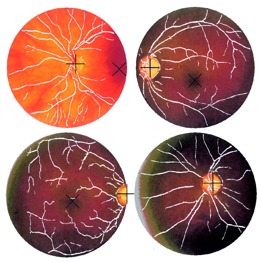
A sample of images showing the results of the recognition of the main components from digital fundus colour images.
VALIDATION OF THE ACCURACY OF DETECTION OF REGIONS
An experienced ophthalmologist observed the localisation of the optic disc and fovea by the algorithms. In order to provide independent test data for the blood vessels, the same ophthalmologist manually traced the vessels of 73 randomly selected patches of 20 × 20 pixels taken from the images. The traced vessels were then compared with the positions of the vessels identified by the neural network. An example of a random patch is shown in Figure 9.

Example of patch of size 20 × 20 pixels used to measure the accuracy of vessels recognition.
Results
The recognition rates for optic disc, blood vessels and fovea were as follows:
- (1)
The optic disc was identified incorrectly in one image. The sensitivity and specificity for optic disc recognition were 99.1% and 99.1% respectively.
- (2)
The recognition rate of blood vessels by the neural network was 99.56% for training and 96.88% for validation data respectively. The sensitivity and specificity of the detection of blood vessels were calculated for each of the 73 patches. The overall sensitivity and specificity for the detection of the blood vessels were 83.3% (SD 16.8%) and 91.0% (5.2%) respectively.
- (3)
To assess the accuracy of recognition of the fovea, the images were separated into three groups: group 1: 71 images presented all of the fovea of within the image. In 60 the fovea was detected correctly (84.5%) but in 11 (15.5%) the fovea was unidentified; group 2: in 29 retinal images the fovea was at the edge of the image but more than half was present on the image. In 18 images the correct position of the fovea was located (62.1%). In one image the fovea was detected inaccurately in the nasal retina (3.4%). The fovea was not identified in 10 images (34.5%); group 3: 12 retinal images either presented no fovea or less than half of the foveal area was within the image. The algorithm did not identify a fovea in these images.
The overall sensitivity and specificity of the detection of the fovea were 80.4% and 99.1% respectively.
Discussion
In this study computer based algorithms were used to detect the main regions of the fundus without any intervention from an operator. The accuracy of the detection was high for the optic disc, blood vessels, and the fovea (especially when the image contained the whole foveal area). It is hoped that the detection of these regions will aid the examination of fundal disorders. The optic disc was particularly reliably detected and may be examined in the future for patterns of disease such as glaucoma.36 The fovea was missed in a number of cases but usually when there was poor centration of the fovea in the image. This can be easily remedied by more careful fundus photography. The detection of the major blood vessels was performed using NN analysis. NNs have been employed in the past in other areas of medicine37 and ophthalmology38 39 because of the capability of these programs to cope with highly variable images. Indeed, NN have already been used before to detect features of retinopathy but employing minimal preprocessing.40 The preprocessing and post-processing used in this study reduces the reliance upon the NN and improves the efficiency of the computer analysis. The smaller blood vessels were more difficult to detect. However, the method used to calculate the accuracy of the detection of the blood vessels by comparing vessels recognised by the NN technique with the vessels traced by the ophthalmologist may introduce some errors. It was technically difficult for the ophthalmologist to locate subjectively the exact position of vessels, especially at their edges. Therefore, the accuracy of the ophthalmologists’ identification of blood vessels may have been variable. Other methods may need to be explored in order to detect all of the blood vessels—for example, active contour models (SNAKES),41 42 to avoid confusion with features such as retinal haemorrhages. There may be other applications for this technology—for example, the accurate detection of the major blood vessels may allow the “fingerprint” of the blood vessels to be used for identifying individuals in a way similar to that in which iris crypts have been utilised.43
In this study it was possible to detect the main regions of the fundus image. Once these have been identified, the data from these regions can be analysed for abnormality. Of course some of the diseases that we would propose to study may alter the appearance of these regions, reducing their detection. However, the algorithms were designed to minimise this risk, particularly for disease processes such as diabetic retinopathy. In diabetic retinopathy further algorithms will be required to detect features which indicate risk to the patient’s sight such as neovascularisation, cotton wool spots, venous changes, and parafoveal exudation. The detection of other features of retinopathy in diabetes (haemorrhages and exudates), and other disorders such as senile macular degeneration, will be facilitated by the removal from the image data set of complex regional features such as the blood vessels and the optic disc. In diabetes, grading of a patient’s retinopathy by fundus imaging and computer analysis, at the site of acquisition of the image, would allow an immediate opinion for the patient on the urgency of referral for an ophthalmological opinion.
In conclusion, computer algorithms were able to detect regions of the fundus. These may be exploited for the examination of patterns of disease. This may have particular relevance to the management of common ophthalmological disorders such as diabetic retinopathy.
Acknowledgments
We acknowledge the help of Professor Sonksen, Robin Edwards, and Shirley Smith of the Department of Medicine, St Thomas’s Hospital, London, for the use of their images.
Grant support organisation: The Development and Promotion of Science and Technology Talent’s Project (Thailand); Overseas Research Student Awards (UK).
Proprietary interest category: Nil.
colour local contrast enhancement
The RGB colours, whereR, G, andB are abbreviated from the coloursRed, Green, andBlue respectively, represent the colour model used for computer graphics or image analysis. Another colour model, which will be used in this work, is theIHS model, whereI, H, andS are abbreviations forIntensity, Hue, and Saturation respectively. TheRGB and IHS have an invertible relation between them.21
The importance of an RGB model is to display colour images. To present the full colour techniques for image enhancement in some detail, we are interested in theIHS model. TheIHS model is best suited to present full colour techniques for image enhancement in detail. It is important that once the IHS model is applied to enhance an image, it must be converted back to RGB for visual display. The IHS model is suitable for image enhancement because the intensity component is decoupled from the colour information of the image. Applying the local contrast enhancement technique to the intensity component and converting the result to RGB for display will not affect the colour content of the image.
LOCAL CONTRAST ENHANCEMENT44
Let the intensity, f, of the picture elements (pixels) of an N ×N digital image be indexed by (i, j) 1⩽i, j ⩽ N. Consider a subimage of size M ×M centred on (i, j) in this paper M=49. Denote the mean and standard deviation of the intensity withinW by <f>W and ςW(f) respectively.
The objective is to define a point transformation dependent onW such that the distribution is localised around the mean of the intensity and covers the entire intensity range. The implicit assumption is that W is large enough to contain a statistically representative distribution of the local variation of grey levels, yet small enough to be unaffected by the gradual change of contrast between the centre and the periphery of the fundus image. The adaptive contrast enhancement transformation is defined by where the sigmoidal function was
 whilef
max andf
min are the maximum and minimum values of intensity within the whole image with
whilef
max andf
min are the maximum and minimum values of intensity within the whole image with

The local contrast enhancement function provides large contrast enhancement for an initially small ς (poor contrast) and little contrast enhancement for an initially largeς (high contrast).
As a result of local contrast enhancement, the dark area is brighter and clearer showing more detail. However, the technique of local contrast enhancement not only adjusts the contrast of the image but also increases the noise. Hence, a 2D Gaussian smoothing filter or median filter has been applied in order to reduce the noise before the local contrast enhancement process.
prepare data for NN
FIRST PRINCIPAL COMPONENT45
The PCA (principal component analysis) technique is the same as the Karhunen Loeve transform technique, also known as Hotelling transform, which aims to form linear combinations of the image bands in order to maximise the information content in the highest order bands. Giving a set of K image bands, denoted by the intensities of N2 pixelsf
a(i) for i=1,...,N a = 1,...,K. We first form a set of zero mean images by subtracting off the mean of each band
To simplify the formulation, it is convenient to write the set ofK image bandsg
a(i) as a N
2 ×K matrix, where each image of the spectral band forms a column of the matrix normally,
We define a K byK matrix C as
This is the un-normalised correlation between theath and the bth image bands.
Hence C is the spectral correlation matrix of the images. We form a matrix H of uncorrelated images by the orthogonal K ×K matrix transformB. it follows that
  for a =1, ... , K andh
1(1),h
1(2), ... ,h
1(N) will be the first component of the set of principal components which will be used together with the edge gradient as the pattern data for classification by a neural network.
for a =1, ... , K andh
1(1),h
1(2), ... ,h
1(N) will be the first component of the set of principal components which will be used together with the edge gradient as the pattern data for classification by a neural network.
EDGE GRADIENT
In this paper we applied the edge operator to the first component of a PCA image. Canny has defined an edge detection operator, which is optimal for step edges corrupted by white noise. The operator that we use in this work is the implementation of operator obtained by Spacek. The reasons that we use Spacek’s solution because Canny was unable to construct a solution of the defining conditions and so approximated one by a difference of gaussians. Spacek demonstrated that performance of his solution was superior to Canny’s approximation. Since the operator satisfies the conditions proposed by Canny we refer to it as the Canny edge operator.
The Spacek method that we use takes the form.28
The response an image to an edge kernel is given by a 2D discrete convolution, the edge strength in the xdirection
ex
(x,y) = ∑∑hx
(ξ,η)f(x−ξ,y−η)dξdη (B12) with a similar equation fore
y(x, y). The intensity of the edge image intensity is defined by
post-processing
AREA
The simplest and most natural property of a region is its area, given by the number of pixels of which the region is comprised. This method was used to remove the small regions of the output vessels/non-vessels classification from neural net, small regions with less than 30 pixels were removed.
COMPACTNESS33
Compactness is a commonly used shape descriptor independent of linear transformations given by
ELLIPSE PARAMETER
The ellipse parameter used is the ratio between the major and the sum of the two (major and minor) axes of an ellipse. This parameter describes the shape of the region and lies between 0.5 (a circle) and 1 (a line). The method that we used to calculate this parameter is the same as employed in PCA. Considering a region, with two variables, x variable (positions of the region pixels in xcoordinate) and y variable (positions of the region pixels in y coordinate). The major and minor axes of the region can be calculated as the eigen values of the covariance matrix: wherex
i,y
i are coordinates in thex, y directions of the region and <x>, <y> are the average value of the region’sx, y coordinates. From this property, the ellipse parameter of circle, ellipse, and line are 0.5, 0.5 < ellipse param <1, and 1 respectively. From our experiments with the test images of variable shapes, we decided to use an ellipse parameter of less than 0.95 the small regions (less than 100 pixels) to classify then as non-vessels.
wherex
i,y
i are coordinates in thex, y directions of the region and <x>, <y> are the average value of the region’sx, y coordinates. From this property, the ellipse parameter of circle, ellipse, and line are 0.5, 0.5 < ellipse param <1, and 1 respectively. From our experiments with the test images of variable shapes, we decided to use an ellipse parameter of less than 0.95 the small regions (less than 100 pixels) to classify then as non-vessels.