Article Text

Abstract
AIMS To evaluate the reproducibility of the retardation values (change in polarisation) obtained with the scanning laser polarimeter in a series of normal subjects and glaucoma patients. To improve the analysis of the raw data by devising and evaluating a blood vessel removal algorithm.
METHODS Scanning laser polarimetry was performed on 10 normal subjects and 10 glaucoma patients. A series of six images was obtained from each eye. The normal subjects were re-imaged 3 months after their initial assessment. The retardation values obtained from each eye were analysed using the authors’ own methods, including the use of an algorithm to remove blood vessels from the polar profiles. The reproducibility of these measurements and the performance of the blood vessel removal algorithm were assessed.
RESULTS The “individual point” coefficient of variation was approximately 12.5% for normal subjects and 17.0% for glaucoma patients. The “integral” coefficient of variation for these groups was approximately 5.5% and 9.5% respectively. The reproducibility of the measurements did not improve with an increased number of measurements. There was no difference in the reproducibility of the measurements in normal subjects over time. The blood vessel removal algorithm improved the reproducibility of the measurements when the shape of the profile was assessed.
CONCLUSION The intraoperator reproducibility of retardation values obtained with the scanning laser polarimeter is satisfactory for its use as a clinical tool. The use of a blood vessel removal algorithm improves the reproducibility of the measurements and also assists the clinician in the interpretation of the polar profiles. Furthermore, it allows the construction of normal database polar profiles, thereby enabling the identification, location and quantification of retinal nerve fibre layer damage in an “at risk” individual’s polar profile.
- scanning laser polarimetry
- glaucoma
- reproducibility
- algorithm
Statistics from Altmetric.com
The retinal nerve fibre layer is the innermost layer of the retina and consists of retinal ganglion cell axons. In glaucoma, this layer undergoes localised or diffuse thinning resulting in a subsequent loss of visual field. The examination of the retinal nerve fibre layer is considered to be essential for the diagnosis and monitoring of patients with glaucoma. Furthermore, this assessment can provide an early indication of the presence of glaucoma,1 2 unlike visual field analysis which may only detect an abnormality when up to as much as 50% of the retinal nerve fibre layer has been lost.3
The traditional clinical examination of the retinal nerve fibre layer involves red-free ophthalmoscopy and photography.4Unfortunately, both of these techniques are subjective and predominantly qualitative in nature. However, in recent years, new computerised image analysing techniques have been developed5 6 in an attempt to provide a more reliable, objective and quantitative measurement of the retinal nerve fibre layer.
Scanning laser polarimetry is one of these new techniques.7 It utilises the properties of polarised light to measure the thickness of the birefringent retinal nerve fibre layer.8 The underlying principle assumes that the birefringence of the retinal nerve fibre layer causes a change in the state of the polarised light (known as retardation). This retardation is measured by the instrument and converted into a measure of the retinal nerve fibre layer thickness based upon the assumption that there is a linear relation between the thickness and optical properties of this layer.8
Currently, initial reproducibility9 10 and age-effect findings10 11 with this new technology have been reported. Furthermore, studies have also assessed the retardation values obtained from a population of normal and glaucomatous subjects,11 as well as comparing retardation values with visual field loss12 and with standardised photography.13 However, no study has attempted to improve the interpretation of the raw data obtained with the scanning laser polarimeter (“Nerve Fiber Analyzer”, Laser Diagnostic Technologies, Inc, San Diego, CA, USA). In this study, a method for improving the interpretation of the raw data is described. Furthermore, the reproducibility of these data (retardation values) obtained from a small population of normal and glaucoma patients is determined.
Patients and methods
SUBJECTS
Ten normal subjects with healthy eyes were examined along with 10 patients with primary open angle glaucoma recruited from the glaucoma clinics at Bristol Eye Hospital. The age range for the normal group was 32–68 years and the glaucoma group was 45–72 years. This reproducibility study was approved by the ethics committee for the United Bristol Healthcare Trust and informed consent was obtained from all of the subjects.
Normal subjects were included in the study if there was no family history of glaucoma and they had had no intraocular pressure rise or ocular trauma in the past, a best corrected visual acuity of 6/12 or better, normal anterior segments on slit lamp biomicroscopy, intraocular pressure of less than 22 mm Hg (Goldmann tonometer), normal optic nerve head appearances on stereoscopic optic disc photography, and no glaucomatous visual field defects on Humphrey 24-2 full threshold automated perimetry.
Primary open angle glaucoma patients were included if they had a best corrected visual acuity of 6/12 or better, anterior segment examination which confirmed open angles but did not demonstrate pseudoexfoliation or pigment dispersion, glaucomatous changes to the appearance of their optic nerve heads on stereoscopic optic disc photography, and had visual field abnormalities consistent with glaucoma. These visual field defects were defined by at least three adjacent points 5 dB or more below the normal with a Humphrey 24-2 full threshold program.
SCANNING LASER POLARIMETER
Retardation was measured with a Mark I scanning laser polarimeter (“Nerve Fiber Analyzer” (NFA I)).14 The instrument is based upon a scanning laser ophthalmoscope with a polarisation modulator, corneal polarisation compensator and polarisation detection unit integrated into the system. A near infrared diode laser (wavelength of 780 nm) is used as the light source and its polarisation state modulated. The laser beam is focused onto a point on the retina by the ocular optical media. The light then undergoes refraction by the birefringent retinal nerve fibre layer, reflection by the deeper retinal layers, and further refraction before emerging from the eye in a different state of polarisation. This emergent beam is separated from the incident light by a non-polarising beam splitter before being analysed by the instrument’s polarisation detection unit. The output from the detection unit is stored in the memory of the accompanying microprocessor.
The scan head enables the illumination of an area of retina ranging from 10 to 20 degrees. In this study a 15 degree field of view was utilised and the illuminating laser beam was subsequently deflected to all positions encompassing this field to enable the previous process to occur. The “gain” of the polarisation detection unit can be modified through the “intensity dial” situated on the scan head. An image consists of 256 × 256 pixels and the retardation data for these 65 536 retinal positions is collected in 0.7 seconds. This includes the activation of the proprietary corneal polarisation compensator which neutralises the effects of the birefringent cornea. The microprocessor uses an algorithm to convert the retrieved retardation data from each measured position into a retardation map (image) which displays the state of polarisation at each location within the field of view. This takes approximately 15 seconds and can be displayed in a variety of pseudocolour coded scales.
The retardation values can be retrieved from the image by defining an elliptical or circular zone of interest within the peripapillary region. Currently there is no standard method for retrieving these data. In this study, the optic disc margin of each eye was defined by placing a circle around the inner margin of the peripapillary scleral ring by a single experienced operator. Retardation values were subsequently obtained for six circles ranging from 1.5 to 2.0 disc diameters in dimension at 0.1 disc diameter increments. For each circle, the “band width” function was set at 1 and the “sector” function set to 360. In essence, this means that for each of the degrees comprising a circle of data, only one retardation value was used for each angular degree.
The retardation values obtained by the above method were transferred from the integrated microprocessor to a personal computer for further calculation. A polar coordinate plot (polar profile) (see Fig 1) was calculated for each eye by obtaining a mean retardation value for each of the 360 degrees. This mean value derives from the average of the retardation values obtained at each angular degree for the six circles from 1.5 to 2.0 disc diameters in dimension.

Example of a polar profile of a normal subject.
REPRODUCIBILITY STUDY
In this study, each of the 10 normal subjects and 10 glaucoma patients had six images obtained from each eye during a single imaging session. Furthermore, the 10 normal subjects were also examined on one more occasion 3 months after their initial assessment. The imaging of all subjects and patients was performed in a dimly lit room through undilated pupils by a single experienced operator (AW). The “intensity dial” was reset for each image in an attempt to obtain the optimum use of the dynamic range of the polar profiles. In essence, this requires the operator to adjust the dial until a few “blue speckles” are observed on the liquid crystal display, a procedure which is documented in the NFA I user’s manual. In all imaging sessions, the patients rested after each image acquisition and subsequently repositioned themselves for each further image.
The polar profiles obtained from each eye of all subjects were analysed in the following way on a personal computer separate to the integrated microprocessor of the scanning laser polarimeter. The first three polar profiles from each subject were initially aligned using the author’s own “best fit” algorithm based upon a “least squares” method. In brief, this algorithm comprises the calculation of the sum (designated “s”) of the square of the differences in retardation values at each of the 360 points comprising a polar profile for a specified alignment of the three polar profiles. The alignment of the three profiles is then modified in a systematic fashion and the process repeated. The alignment with the lowest “s” value is defined as having the “best fit”.
A mean polar profile was subsequently created from these three aligned profiles. This process was repeated for each eye using the first four, first five and all six images, along with the series of three images obtained from each of the normal subjects 3 months after their initial assessment. In each case, an appropriate best fit algorithm was used to align the polar profiles and a mean profile was created for each of the groups of profiles being assessed.
The reproducibility of these profiles was measured by determining the coefficient of variation (COV) (standard deviation divided by the mean and expressed as a percentage) for each of the 360 degrees comprising a polar profile. The mean COV for a polar profile was calculated by obtaining the average COV for the 360 individual COVs. This calculation was performed on all subjects to obtain mean COVs for each of the four groups of profiles assessed (that is, the first three, first four, first five, and all six profiles).
The results of this aspect of the study are presented in Tables 1 and2. Table 1 illustrates the average range of COVs obtained from the individual 360 degrees comprising the polar profiles of the normal and glaucoma subjects. Table 2 illustrates the overall mean COVs obtained for the 10 normal subjects and 10 glaucoma patients at each of the various groups of profiles assessed. The interquartile range of the mean COVs for the appropriate groups are also illustrated.
Mean values for the range of the 360 individual COVs for the groups of normal and glaucoma subjects
Reproducibility for normal and glaucoma subjects (individual point analysis)
This evaluation of the instrument’s reproducibility is different from other reported values9-11 which assess the reproducibility of the “integral” or area under the profile rather than the reproducibility at each “individual point” comprising a polar profile. In an attempt to enable a comparison with other reported measurements, the reproducibility of the polar profiles has also been calculated by obtaining integral values for each polar profile and subsequently determining the COV for the integrals of the first three, first four, first five, and all six images. These results are demonstrated in Table 3 and are in the same format as Table2.
Reproducibility for normal and glaucoma subjects (integral analysis)
BLOOD VESSEL REMOVAL ALGORITHM
The presence of blood vessels within the polar profiles has been observed to be a source of high measurement variability by the authors and also an area where the interpretation of the profile is made more complex.15 Figure 2 is an illustration of a retardation image of a normal subject with the retardation values at each of the 360 locations plotted as a circumferential polar profile. The higher retardation values are expressed as greater distances from the concentric circular band (the sampling zone). It can be seen that this polar profile and its linear graphical form (see Fig 1) are made more difficult to analyse because of the presence of lower retardation values (troughs) at the sites of blood vessels.
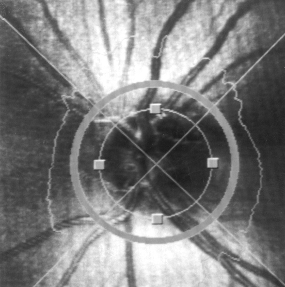
An illustration of a retardation image of a normal subject demonstrating the location and size of the concentric sampling zone used in this study. The circumferential polar profile is also demonstrated (see main text for details).
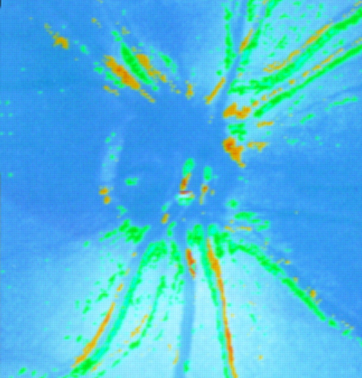
Figure 3 illustrates a comparison map compiled by the NFA I software of two retardation images of the same eye of a normal subject taken within 2 minutes of each other by the same operator (AW). The yellow and green regions reflect areas of statistically significant change in the retardation values obtained in these areas. This subject is unlikely to have had such extensive retinal nerve fibre layer loss during this short period of time and so these changes probably reflect image alignment inaccuracies and changes within the blood vessel diameters during the acquisition of these two images.

An illustration of a comparison map of compiled by the NFA I software of two retardation images of the same eye of a normal subject taken within 2 minutes of each other by the same operator (AW). The yellow and green regions reflect areas of statistically significant change in the retardation values obtained from these locations.
As a consequence of these observations, the author (AW) has devised an algorithm which removes the blood vessels from the polar profiles without oversmoothing the rest of the profile. The algorithm is designed to detect blood vessels within the profile by assessing gradient changes within the profile. If the threshold for a gradient change is exceeded, the algorithm recognises this as the presence of a blood vessel. The algorithm extrapolates across the region defined by the above process as the site of a blood vessel. This process is performed on several occasions, initially assessing the profile in a clockwise (1 to 360 degrees) and then anticlockwise direction (360 to 1 degree). The presence of vessel bifurcations and trifurcations is also recognised and this requires further processing of the profiles by this algorithm using different gradient thresholds depending upon the nature of the vessel composition. Full details outlining the blood vessel removal algorithm are documented in the . A polar profile demonstrating the effect of the blood vessel removal algorithm on the profile of a normal subject is demonstrated in Figure 4.

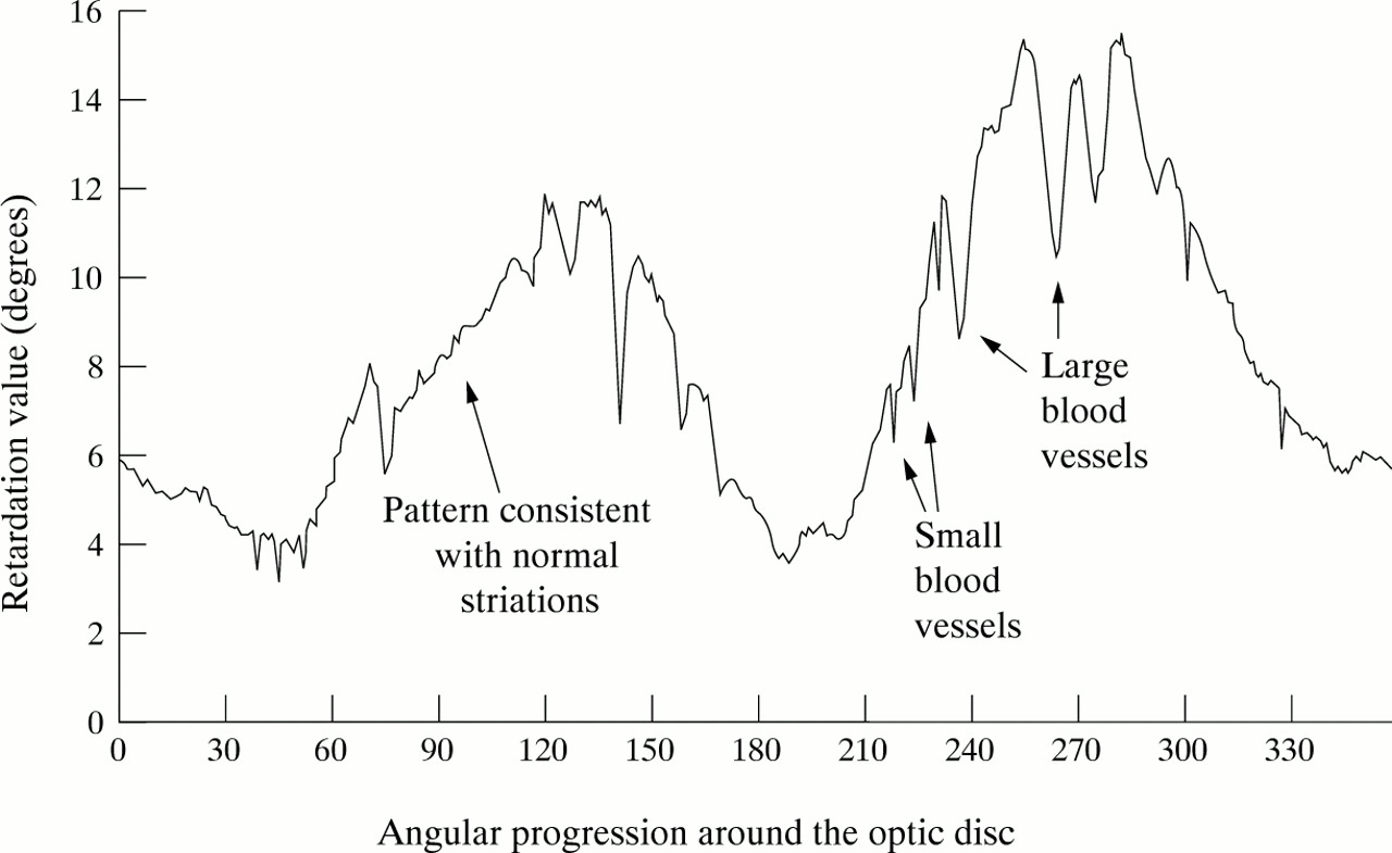
Example of a polar profile of a normal subject demonstrating the effect of the application of the blood vessel removal algorithm. The blood vessel removed polar profile is illustrated by the solid line, while the original polar profile containing the blood vessels is illustrated by the broken line.
The performance of this algorithm has been assessed using the small series of 10 normal subjects and 10 glaucoma patients. Three polar profiles from each subject were initially aligned using the author’s own best fit algorithm as described previously. The reproducibility of these profiles was measured by determining the mean COV for a profile as described above. The same three polar profiles from each subject subsequently underwent further analysis using the blood vessel removal algorithm. The resultant “blood vessel free” profiles were aligned using the same best fit algorithm. The reproducibility of these profiles was measured in the same manner as described for those profiles with the blood vessels intact. The results of this aspect of the study are presented in Table 4 and illustrate the overall mean COVs obtained for the 10 normal subjects profiles and 10 glaucoma patients profiles with and without the blood vessel removal algorithm. The interquartile range of mean COVs for the appropriate groups are also illustrated.
Blood vessel removal algorithm performance (individual point analysis)
The shape of a polar profile can be described by evaluating the gradient changes between the 360 points comprising an individual profile. One method of calculating this variable is to obtain the difference in retardation value between two adjacent points and subsequently derive a “gradient” value for all 360 degrees. The shapes of the polar profiles of all of the “aligned” images (with and without blood vessels) were calculated using this method. The reproducibility of the profile shape variable was measured by initially determining the standard deviation for each of the 360 gradient values comprising a polar profile. The mean deviation was subsequently used to express the reproducibility of the “shape” variable and this was calculated by obtaining the average of the 360 individual standard deviations. These results are demonstrated in Table 5 and are in the same format as Table 4.
Blood vessel removal algorithm performance (profile shape analysis)
STATISTICAL ANALYSIS
One eye from each of the subjects was randomly chosen and used in the analysis of all aspects of this study. Simple descriptive analysis was used to compare the results obtained from the normal and glaucoma groups as well as to compare the performance of the blood vessel removal algorithm in both the normal and the glaucoma group of patients.
Results
Table 1 gives an illustration of the range of measurement variation that is obtained from the 360 individual degrees comprising a polar profile. In both the normal and the glaucomatous groups, the average range of COVs are similar. On an individual subject basis, the maximum COV for an individual degree can be as much as 70%. Table 2illustrates the reproducibility of the polar profiles in the normal and glaucoma groups using the “individual point” analysis. The mean COV for the normal was of the order of 12.5%, while the glaucoma patients had a mean COV of approximately 17%. There was very little reduction in the reproducibility of the measurements obtained for the initial three profiles and the repeat series of three profiles taken 3 months later in the normal subject group. A comparison of the reproducibility of the measurements obtained in the normal and glaucoma groups reveals a 35%–40% increase in measurement variability in the glaucoma patients.
Table 3 illustrates the reproducibility of the polar profiles in the normal and glaucoma groups using the “integral” or “area under the profile” analysis. The mean COVs for the normal and glaucoma groups were approximately 5.5% and 9.5% respectively. There is only a minimal increase in the reproducibility of the measurements obtained for the initial three profiles and the repeat series of three profiles taken 3 months later in the normal subject group. However, a comparison of the reproducibility of the measurements obtained in the normal and glaucoma groups reveals a substantial 70%–85% increase in measurement variability in the glaucoma patients.
Table 4 illustrates the performance of the blood vessel removal algorithm on the reproducibility of the polar profiles in the normal and glaucoma groups using the “individual point” analysis. The mean COV before the application of the algorithm for normal subjects was 11.2% and 16.0% for glaucoma patients. The mean COVs improved by approximately 8%–10.3% and 14.7% respectively after the blood vessel removal algorithm was applied.
Table 5 illustrates the performance of the blood vessel removal algorithm on the reproducibility of the polar profiles in the normal and glaucoma groups using the “profile shape” analysis. The mean deviation before the application of the algorithm for normal subjects was 1.85 and 1.72 for glaucoma patients. The mean deviations improved by two thirds of their original values to 0.56 and 0.62 respectively after the blood vessel removal algorithm was applied.
The location of the improvement in the reproducibility was observed to occur primarily at the edges of the blood vessels. This is demonstrated graphically in Figure 5 which shows a polar profile of a normal subject and the mean deviations for the shape of this profile at each of the 360 points comprising the profile. The mean deviations illustrated are for both before and after the application of the blood vessel removal algorithm on this profile. The areas of greatest reduction in mean deviation are found at the edges of the blood vessels, while the other areas show no significant change in the shape of the profile.
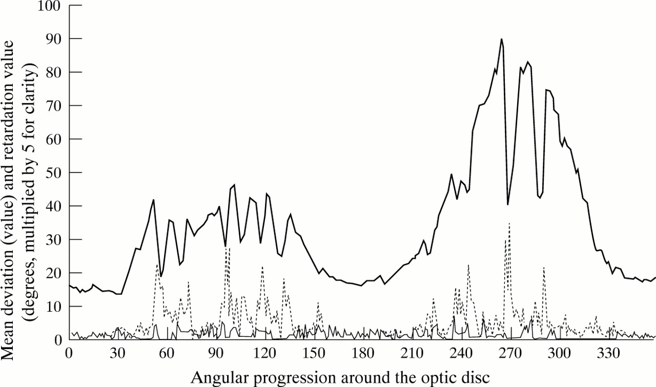
A polar profile of a normal subject with an illustration of the areas of greatest measurement variability in the shape of this profile. The polar profile (retardation values multiplied by five for clarity) is illustrated by the solid bold line. The variability of the profile shape at individual locations is illustrated by the broken line (before the application of the blood vessel removal algorithm) and by the fine line (after the application of the algorithm).
Discussion
The retardation images of normal subjects demonstrate greatest retardation values in the superior and inferior regions, a known feature of the histology of the retinal nerve fibre layer16 and an observation which has been documented previously.11 However, there are also some features in a retardation image which do not reflect known histological patterns of the retinal nerve fibre layer. The most noticeable is the fact that the maximum retardation values are measured in a zone extending from 1.5 to 2.0 disc diameters from the disc margin (data not presented),17 with values at the histologically thicker optic disc margin being lower than in this defined zone.
This discrepancy may be explained by the fact that the scanning laser polarimeter measures the changes in the properties of polarised light which will be maximal when the incident laser light is perpendicular to the microtubular structures within the retinal nerve fibre layer. The complex and diverse arrangement of nerve fibres at the optic disc margin is such that this requirement may not be met, a hypothesis also put forward by other researchers.11
This observation infers that this instrument is measuring relative retinal nerve fibre layer thickness. Furthermore, the interpretation of the polar profile integral (area under the profile) with respect to the distance from the optic disc margin is made more complex. For this reason, it was decided that the retardation values should be sampled from a zone which will enable the observer to retrieve the maximal separation of retardation peaks and troughs. This sampling zone does rely on disc diameters as the measurement variable, but in our study the variation in optic disc size did not present a problem. It was also decided that the retardation values should be analysed at a high frequency of one retardation value per angular degree, as this would enable the retrieval of far more information from the retardation images than the guidelines for the use of the current software.
The mark I version of the scanning laser polarimeter (NFA I) requires the operator to vary the gain of the polarisation detection unit by using an “intensity dial”. This may be a potential source of great measurement variability and may provide the user with difficulties in comparing one image with another. It has been demonstrated by the authors that within the scanning range used for clinical purposes the properties of the intensity dial are linear in nature (data not presented),17 thereby allowing data to be compared through a simple linear transformation process.
The mean COV for individual point measurements of a polar profile were of the order of 12.5% for normal subjects and 17% for glaucoma patients. These values appear to be repeatable over time, as reflected in the repeat series of images performed on the normal subjects. The slight improvement from 12.3% to 11.6%, although not substantial, may reflect an improvement in the operator’s skill in obtaining good quality images. The greater values obtained for the glaucoma group almost certainly reflect the difficulty in achieving even illumination of the peripapillary retina in eyes in which there is an abnormal retinal nerve fibre layer. This finding may be important clinically, especially when it comes to detecting change in the retinal nerve fibre layer thickness.
The individual point reproducibility values appear rather disappointing when compared with other studies.9-11 However, these have not used as sensitive a measure of the retinal nerve fibre layer, but instead have concentrated on evaluating the reproducibility of the area under the profile (or “integral”). Our integral mean COV values of 5.5% and 9.5% for the normal and glaucoma groups are similar to those obtained by other studies10 11 using the mark I scanning laser polarimeter. Although this measurement is more clinically applicable with regard to its reproducibility, it does have the disadvantage of not being as sensitive to more focal and subtle retinal nerve fibre layer defects.
There is little evidence regarding the number of images of an eye that are required to give reproducible results. A study using a scanning laser ophthalmoscope demonstrated that there was no substantial improvement in the reproducibility of the measurements by obtaining more than three images per eye.18 Our results (Tables 2and 3) indicate a similar finding for the scanning laser polarimeter. In all instances apart from the integral mean COV values for glaucoma patients, the COV appeared to get slightly worse if more than three images were used in the measurement of the retinal nerve fibre layer thickness.
The blood vessel removal algorithm has been devised on the observation that blood vessel wall margins are defined in a retardation image by very sharp and well delineated gradient changes. The algorithm is therefore capable of detecting all sizes of blood vessels within a polar profile. A subjective evaluation of the performance of this algorithm has been performed by comparing the “blood vessel removed” polar profiles with stereo optic disc photographs of the same eyes. In this current study, all of the blood vessels from all polar profiles were removed. A much larger study17assessing the polar profiles from over 60 normal subjects has demonstrated this algorithm to be successful in removing 98% of all of the blood vessels from all of the polar profiles.
The assessment of the effect of the algorithm on the individual point reproducibility in a profile reveals a minimal improvement for both normal subjects and glaucoma patients (Table 4). This reduction in the reproducibility of individual point measurements highlights the inherent “noise” that is present at the edges of the vessels within a profile, even though the profiles have been aligned with each other. This can cause substantial “individual degree” measurement variability, as illustrated in Figure 3 and can be of the order of 70%.
It is also possible that this algorithm could be inadvertently smoothing out the fine striations and slit-like “pseudo defects” seen in red-free photography of the retinal nerve fibre layer of normal subjects.19 Although this was not formally assessed in this study, another study20 evaluating red-free photographs and NFA I polar profiles has shown that the normal striations seen photographically appear to produce a polar profile pattern similar to that demonstrated in Figure 1. This pattern is different from that caused by blood vessels (see Fig 1) and is generally left unaltered by the algorithm (see Fig 4). However, the presence of these normal striations or even pathological slit-like defects in the retinal nerve fibre layer adjacent to the blood vessel wall margins may be smoothed over by the extrapolation process performed by the algorithm.
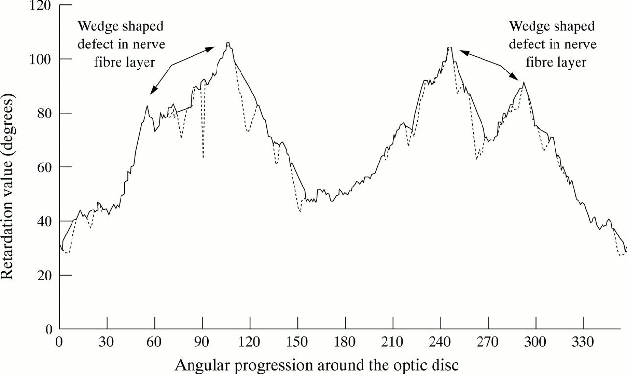
Arguably, a more important clinical variable is the shape of the profile as this may enable the best detection of both localised and diffuse nerve fibre layer defects. The gradient changes and the profile patterns observed for focal wedge-shaped nerve fibre layer defects seen in patients with glaucoma are substantially different from those observed for the blood vessel margins.17 In the initial evaluation of the blood vessel removal algorithm, much attention was focused on the ability of the gradient thresholds to not detect focal wedge-shaped defects. The current gradient thresholds set on this algorithm (see ) were derived from many trials on polar profiles obtained from patients with focal and diffuse nerve fibre layer defects, as well as normal subjects. An example of a polar profile with two types of focal wedge-shaped nerve fibre layer defects is illustrated in Figure 6.
Example of a polar profile of a glaucoma patient with focal wedge-shaped nerve fibre layer defects in both hemiretinas. The blood vessel removed polar profile is illustrated by the solid line, while the original polar profile containing the blood vessels is illustrated by the broken line. The wedge-shaped defects have not been removed by the algorithm.
The assessment of profile shape variability on an individual point basis reveals a substantial two thirds improvement in reproducibility after the application of the blood vessel removal algorithm (Table 5). Figure 5 illustrates the location of this improved reproducibility to be at the edges of the blood vessels, even though all of the images have been aligned with each other. Furthermore, there is no improvement in the variability outside these areas, suggesting that this algorithm is not overtly oversmoothing the rest of the polar profile.
The mark II version of the scanning laser polarimeter (NFA II) and the more recently available GDx (Laser Diagnostic Technologies, Inc, San Diego, CA, USA) have been designed without an intensity dial by utilising a polarisation detection unit which assesses all aspects of the emerging polarised light. Although this may further improve the intra and interobserver reproducibility, we are unaware of any attempt to overcome the difficulty in obtaining even retinal illumination in patients with abnormal nerve fibre layers. As demonstrated in this small study, this may cause significant variations in the retardation values obtained and could be overlooked by solely assessing the integral measurement variability.
This study also demonstrates that the application of a blood vessel removal algorithm to the retardation data has no deleterious effects on the reproducibility of the measurements. However, its application may greatly assist in the interpretation of the profiles, especially if variables such as profile shape are considered to be important. The removal of blood vessels from the polar profile also enables the creation of normal database polar profiles. By using one angular degree datum intervals, the identification of the presence of any retinal nerve fibre layer damage, along with the exact location of this damage and a quantification of the defect is made possible.
The scanning laser polarimeter is an exciting new method for quantifying retinal nerve fibre layer thickness. Up to now, the evaluation of the data obtained with this instrument has not been fully scrutinised. This study highlights some interesting results with the mark I version (NFA I), especially with regard to the design and use of a blood vessel removal algorithm. The removal of the intensity dial and the recent development by the manufacturers of their own blood vessel removal algorithm21 should greatly enhance the reproducibility of the measurements and the interpretation of the data retrieved with the updated NFA II and GDx versions.
Acknowledgments
The authors would like to acknowledge the work of Mrs Gill Bennerson who performed the optic disc photographic documentation of these patients, along with her advice and support throughout this project. This study was supported by the Special Trustees for the United Bristol Healthcare Trust and the UK Pacesetter Fund.
The authors have no financial or proprietary interest in the scanning laser polarimeter (“nerve fiber analyzer” (NFA I) or Laser Diagnostic Technologies Inc.
BLOOD VESSEL REMOVAL ALGORITHM
A polar profile is composed of 360 numbers (one per degree), starting and finishing at the temporal horizontal midline.
Algorithm
The algorithm calculates the gradient (or difference) between degree (x+1) and degree (x). If the gradient does not exceed a threshold then the algorithm proceeds from degree 1 to degree 360 until it registers any gradients greater than the defined threshold (set at −0.47).
If the threshold is breached, the algorithm registers this as the edge of a blood vessel. It then searches for the inflexion in the gradient change (that is, from negative to positive value) before restarting its scanning for a further negative gradient. The location of the next negative gradient is considered to represent the other edge of the blood vessel and the algorithm subsequently extrapolates a straight line from one edge of the vessel to the other, thereby removing the blood vessel from the profile.
The algorithm continues to scan the profile from 1 to 360 degrees, filling in any blood vessels identified by the defined threshold. The result is an outcome profile for the clockwise direction. The algorithm then rescans the profile in the reverse direction (that is, from 360 to 1 degree), removing any blood vessels in a manner outlined previously and resulting in an anticlockwise outcome profile. The outcome profiles from these two calculations are merged by taking the maximum value calculated for each degree.
The resultant profile is then scanned to identify any residual gradients which surpass a threshold of −0.40. This represents the presence of a bifurcation or trifurcation. The algorithm removes these residual blood vessels in a similar manner to that described previously. The removal of a vessel trifurcation requires the identification of a residual inflexion pattern which exceeds several variables outlining its shape.