Article Text

Abstract
AIM To evaluate the image quality produced by polypseudophakia used for strongly hypermetropic and nanophthalmic eyes.
METHODS Primary aberration theory and ray tracing analysis were used to calculate the optimum lens shapes and power distribution between the two intraocular lenses for two example eyes: one a strongly hypermetropic eye, the other a nanophthalmic eye. Spherical aberration and oblique astigmatism were considered. Modulation transfer function (MTF) curves were computed using commercial optical design software (Sigma 2100, Kidger Optics Ltd) to assess axial image quality, and the sagittal and tangential image surfaces were computed to study image quality across the field.
RESULTS A significant improvement in the axial MTF was found for the eyes with double implants. However, results indicate that this may be realised as a better contrast sensitivity in the low to mid spatial frequency range rather than as a better Snellen acuity. The optimum lens shapes for minimum spherical aberration (best axial image quality) were approximately convex-plano for both lenses with the convex surface facing the cornea. Conversely, the optimum lens shapes for zero oblique astigmatism were strongly meniscus with the anterior surface concave. Correction of oblique astigmatism was only achieved with a loss in axial performance.
CONCLUSIONS Optimum estimated visual acuity exceeds 6/5 in both the hypermetropic and the nanophthalmic eyes studied (pupil size of 4 mm) with polypseudophakic correction. These results can be attained using convex-plano or biconvex lenses with the most convex surface facing the cornea. If the posterior surface of the posterior intraocular lens is convex, as is commonly used to help prevent migration of lens epithelial cells causing posterior capsular opacification (PCO), then it is still possible to achieve 6/4.5 in the hypermetropic eye and 6/5.3 in the nanophthalmic eye provided the anterior intraocular lens has an approximately convex-plano shape with the convex surface anterior. It was therefore concluded that consideration of optical image quality does not demand that additional intraocular lens shapes need to be manufactured for polypseudophakic correction of extremely short eyes and that implanting the posterior intraocular lens in the conventional orientation to help prevent PCO does not necessarily limit estimated visual acuity.
- polypseudophakia
- nanophthalmia
- ray tracing analysis
Statistics from Altmetric.com
In 1993, Gayton and Sanders1 first described the use of multiple implants in a case of microphthalmos where the SRK/T formula indicated that a +46D intraocular lens power was required. Since this power was beyond the range available from manufacturers, two lenses were implanted, one in the capsular bag and the second in the ciliary sulcus. The resulting refraction still found the patient +8D hypermetropic—an effect later coined by Holladayet al 2 as the “hypermetropic surprise” in polypseudophakia. An increase in total intraocular lens power of more than 5D over the SRK/T value was subsequently needed to achieve emmetropia. Gayton and Sanders concluded that a single lens would be preferable because of the problems in using current intraocular lens power formulas for these unusually short eyes. Errors in power formulas for extremely short eyes have since been addressed by Holladay.3
Since Gayton and Sanders first published their results on polypseudophakia, Holladay et al 2 and Shugar et al 4 have reported the use of “piggyback” lenses in extremely short eyes. In both cases the authors commented that an even power split should help to reduce the spherical aberration. Shugar et al also used acrylic lenses that were thinner. This theoretically helped to alleviate errors in calculated intraocular lens power and to minimise aberrations further. However, to our best knowledge, no analysis has been performed on the optical quality produced by multiple implants.
The aim of this paper was therefore to show whether the current practice of using multiple intraocular lens implants gives an equivalent or superior optical performance to a single intraocular lens in extremely short eyes. An answer to this question would allow surgeons and manufacturers to make an informed choice as to whether to use single high power intraocular lenses or whether refinement of the procedures for using currently available lenses for extremely short eyes is appropriate.
Methods
AXIAL IMAGE QUALITY
Axial image quality must be considered of prime importance because it can limit the maximum attainable visual acuity assuming normal retina/brain function. If it is assumed that the crystalline lens is rotationally symmetric (it has been shown that asymmetries make little difference to the paraxial properties and aberrations5), then the only aberration affecting axial image quality is spherical aberration once emmetropia has been achieved. There are few data on the spherical aberration of the human crystalline lens. Results that have been reported suggest that the lens has approximately zero spherical aberration,6 a large negative amount of spherical aberration,7 and a positive contribution.8 In a more recent study by Sivak and Kreuzer,9 both positive and negative values were found. In view of this conflicting evidence it would seem appropriate to minimise the spherical aberration contribution of any implant lens.
For a single, spherically surfaced implant lens, the factors affecting the spherical aberration are power, lens shape, optical diameter of the lens, refractive index, and conjugate ratio (the relative position of the object and image). It would appear, therefore, that there are a number of variables that can be used to control spherical aberration. However, a cursory consideration removes most of them: the lens power is fixed to achieve emmetropia; the used lens diameter is fixed by the pupil size which obviously varies (it is therefore necessary in the following analysis to set a reasonable pupil size and to leave it constant for the different designs evaluated); and for a fixed corneal power and implant lens power, the conjugate ratio is determined. This leaves only the lens shape and refractive index as variables that can be used to control spherical aberration. With double implant lenses, the number of factors that can be varied to control spherical aberration is increased. They are the lens power split, the shape factors of both lenses, and the refractive index of the material.
LENS POWER SPLIT
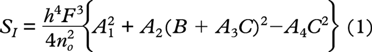
The primary spherical aberration of a thin lens is given by10:

where h is the lens semidiameter (paraxial marginal ray height at the lens), no is the refractive index in which the lens is immersed, F is the paraxial lens power, B is the lens shape factor, and C is the conjugate ratio. These, together with the constants A1 to A4 are all defined in the .
To find the power split between the two implant lenses, which maximises axial image quality, it is necessary to know how spherical aberration varies with power, F. Equation (1) is a third order equation in power and contains terms in F3, F2, and F after substituting for the conjugate ratio. However, the variation in spherical aberration with power is predominantly cubic and therefore we can write
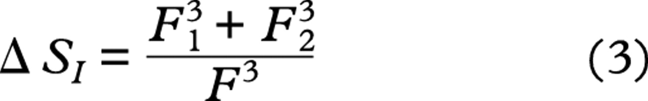
For two thin lenses with powers F1 and F2, the primary spherical aberration produced by each lens is therefore proportional to F1 3 and F2 3 respectively. Primary spherical aberration values can be summed and hence the total primary spherical aberration of the two intraocular lenses is proportional to F1 3 + F2 3. For a single intraocular lens which has the same total power (F=F1+F2), the reduction in spherical aberration, ΔSI, for the two implant lenses compared with the equivalent single lens can be expressed as the ratio

By substituting F2=F−F1 and differentiating with respect to F1, we find that the two implant lenses contribute the minimum spherical aberration when there is an even power split.
An equal power split is optimal irrespective of other variables since the shape of the lenses and the used lens diameters are not affected by the power split provided that the lenses are in contact. Since the lens powers determine the intermediate image locations, the conjugate factors of both lenses are also known.
LENS SHAPE
The lens shape for maximum axial image quality can be found by partially differentiating equation (1) with respect to the shape factor B. Equating the result to zero gives the lens shape factor for minimum spherical aberration as
For a known conjugate factor for each lens, equation (4) gives the shape factor to achieve minimum spherical aberration. The thin lens contributions for primary spherical aberration can be summed, hence minimising the spherical aberration of both lenses independently will produce the best overall result.
CALCULATION OF SPHERICAL ABERRATION
The equations derived above can be used to calculate the optimum lens variables for any specified eye. The specifications of the two eyes used in the calculations presented in this study have been taken from Holladay et al’s paper.2They include the two categories of eye where polypseudophakia may be useful—high hypermetropes with axial lengths of approximately 19 mm and nanophthalmic eyes with axial lengths around 16 mm. The data for these two example eyes are given in Table 1. From the specification of corneal power, axial length, intraocular lens axial position (for double implants, the two lenses are assumed to be in contact), pupil diameter, and refractive indices it is possible to compute the required power of the intraocular lens(es) by performing a paraxial ray trace. The results of the ray trace also allow the conjugate factors of each implant lens to be calculated from the formula (A2) given in the. Equation (4) is then used to determine the optimum shape factor for each lens. Finally, all of this information can be substituted into equation (1) to find the spherical aberration for each lens and the contributions summed to find the total spherical aberration.
Specification of the hypermetropic example eye (number 1 in the table) and the nanophthalmic eye (number 2) used for the calculations of image quality presented in the text
MTF curves were then computed using a commercial optical design program (Sigma 2100, Kidger Optics Ltd, Crowborough, East Sussex). The intraocular lens variables were calculated as described above and the lenses placed within a Gullstrand–Le Grand schematic eye11 where the corneal asphericity (“p value”) is taken as 0.81. This value is the average of a number of studies on corneal shape.12-19 The pupil size is set at 4 mm (computations were carried out for a pupil diameter of 3.58 mm which accounts for the Stiles–Crawford effect20) and for a single wavelength of 587.6 nm. In all cases the optimum focus was found which maximised visual acuity. This would appear realistic since it corresponds to optimum refraction with subjective confirmation.
OFF AXIS IMAGE QUALITY—OBLIQUE ASTIGMATISM
Off axis image quality is important because it can affect visual performance across the visual field and may limit the extent of the useful visual field. In coaxial systems, off axis image quality is affected by a number of aberrations. Of these, the five primary monochromatic aberrations need consideration first since they tend to be large in optical systems that have not been corrected. These aberrations are—namely, spherical aberration (see previous section), coma, oblique astigmatism, field curvature, and distortion. The latter two are unimportant in the eye since the curvature of the retina minimises the detrimental effect of field curvature and there is evidence from lens induced retinal image geometry changes that compensation for distortion can occur at the higher visual centres.21
Oblique astigmatism is perhaps the most detrimental aberration as far as off axis image quality is concerned. There are also reasonable empirical data about ocular oblique astigmatism that demonstrate that it is well corrected in the average human eye with the tangential and sagittal focal surfaces lying either side of the retina. This places the disc of least confusion approximately on the retina giving the best possible image quality although results show a significant intersubject variation.21 Less is known about coma, although recent results indicate that it may be more important than initially thought owing to the lack of a common axis for the optical surfaces in the eye.22
An implant lens placed at the iris plane will have a constant amount of oblique astigmatism for a given field angle irrespective of lens shape or spherical aberration. If the implant lens is placed away from the iris (considered to be the aperture stop), it is possible to control oblique astigmatism with lens shape.
Primary (third order) astigmatism is given by10:
where the terms have the same meaning as in equation (1). The Lagrange invariant, H, the eccentricity variable, E, and constants A5 and A6, which have not appeared before, are all defined in the . If the astigmatism given by equation (5) is set to zero, a quadratic equation in B results, which can be solved to find the lens shape that produces zero oblique astigmatism (see).
In order to assess the image quality, results were compared against the astigmatism of the modified Gullstrand–Le Grand schematic eye defined in Table 2. The reason for this is to give a baseline measurement of oblique astigmatism which agrees reasonably well with experimental observations and hence to assess the potential advantage of attempting to correct oblique astigmatism. In all cases, the sagittal and tangential image “shells” were computed using a commercial optical design program (Sigma 2100, Kidger Optics Ltd, Crowborough, Sussex, UK) together with our own software developed during the course of this work.
Specification of the modified Gullstrand–Le Grand schematic eye used in this study
Results
AXIAL IMAGE QUALITY
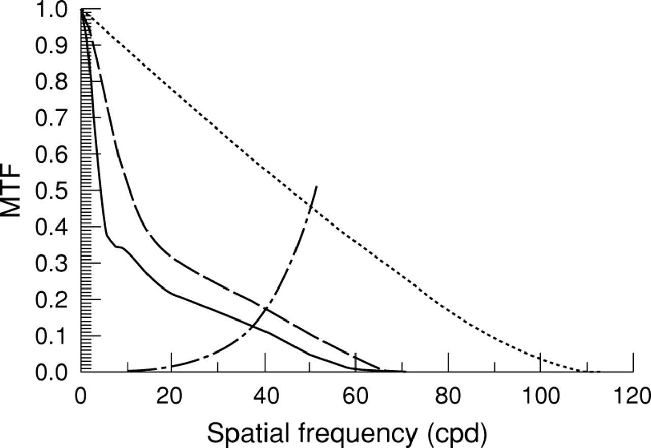
Modulation transfer function (MTF) curves have been used to assess axial image quality. These curves represent the contrast sensitivity of the optics of the eye and implant lenses for increasing spatial frequency. Figures 1 and 2 both demonstrate an improved MTF performance for the double implants compared with a single IOL over a majority of spatial frequencies. To assess this improvement in terms of a clinically measurable variable, visual acuity has been estimated following an approach suggested by Atchison.23 The retina/brain contrast threshold, which was fitted from data for subject FWC in the classic paper by Campbell and Green,24 has been superposed on the MTF curves and the Snellen acuity calculated from the spatial frequency where the curves intersect. For the hypermetrope the estimated Snellen acuity improves from 6/4.3 with a single implant to 6/3.6 for double implants (Fig 1). For the nanophthalmic eye there is also a small improvement in the estimated Snellen ratio from 6/4.8 to 6/4.4 when using double implants (Fig 2).

Axial modulation transfer function (MTF) curves for both a single (solid line) and double implant lenses (broken line) implanted in the hypermetropic example eye described in the text. The dotted curve represents the diffraction limit for a 4 mm pupil size with Stiles–Crawford correction and for a wavelength of 587.6 nm. The retina-brain contrast threshold (alternate dash-dot curve) has been superposed to allow estimates of visual acuity, which occur where the curves intersect, to be made.

Axial modulation transfer function (MTF) curves for both a single (solid line) and double implant lenses (broken line) implanted in the nanophthalmic example eye described in the text. The dotted curve represents the diffraction limit for a 4 mm pupil size with Stiles–Crawford correction and for a wavelength of 587.6 nm. The retina-brain contrast threshold (alternate dash-dot curve) has been superposed to allow estimates of visual acuity, which occur where the curves intersect, to be made.
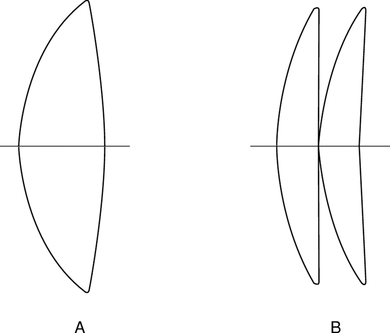
The lens shapes that achieve these results are given in Table 3 and are illustrated in Figure 3. The values in the table can best be appreciated if it is recalled that a value of +1 is a convex-plano lens (convex surface anterior), 0 is an equiconvex lens and −1 is a plano-convex lens. (In the remainder of this paper we shall consistently refer to a lens as convex-plano if its anterior surface is convex and plano-convex if it is oriented such that its posterior surface is convex). Values larger than 1 or less than −1 are meniscus lenses. It can be seen that, for the single implants, the optimum shape is biconvex with the most convex surface anterior in the eye. For both cases of polypseudophakia, the front lens is approximately convex-plano and the second lens meniscus (anterior surface convex). Therefore it is possible to recommend intraocular lens shapes for an eye of given specification which maximise visual acuity. However, lens shape can affect oblique astigmatism causing a change in visual acuity across the field. This will be considered next.
Intraocular lens shape factors for achieving optimum axial image quality (least spherical aberration) and zero primary oblique astigmatism for the two example eyes described in the text using both single and double lens implants

Single and double implant intraocular lens shapes to maximise axial image quality (minimise spherical aberration). Note that the lens shapes are the same for both the hypermetropic eye and the nanophthalmic eye described in the text.
OFF AXIS IMAGE QUALITY—OBLIQUE ASTIGMATISM
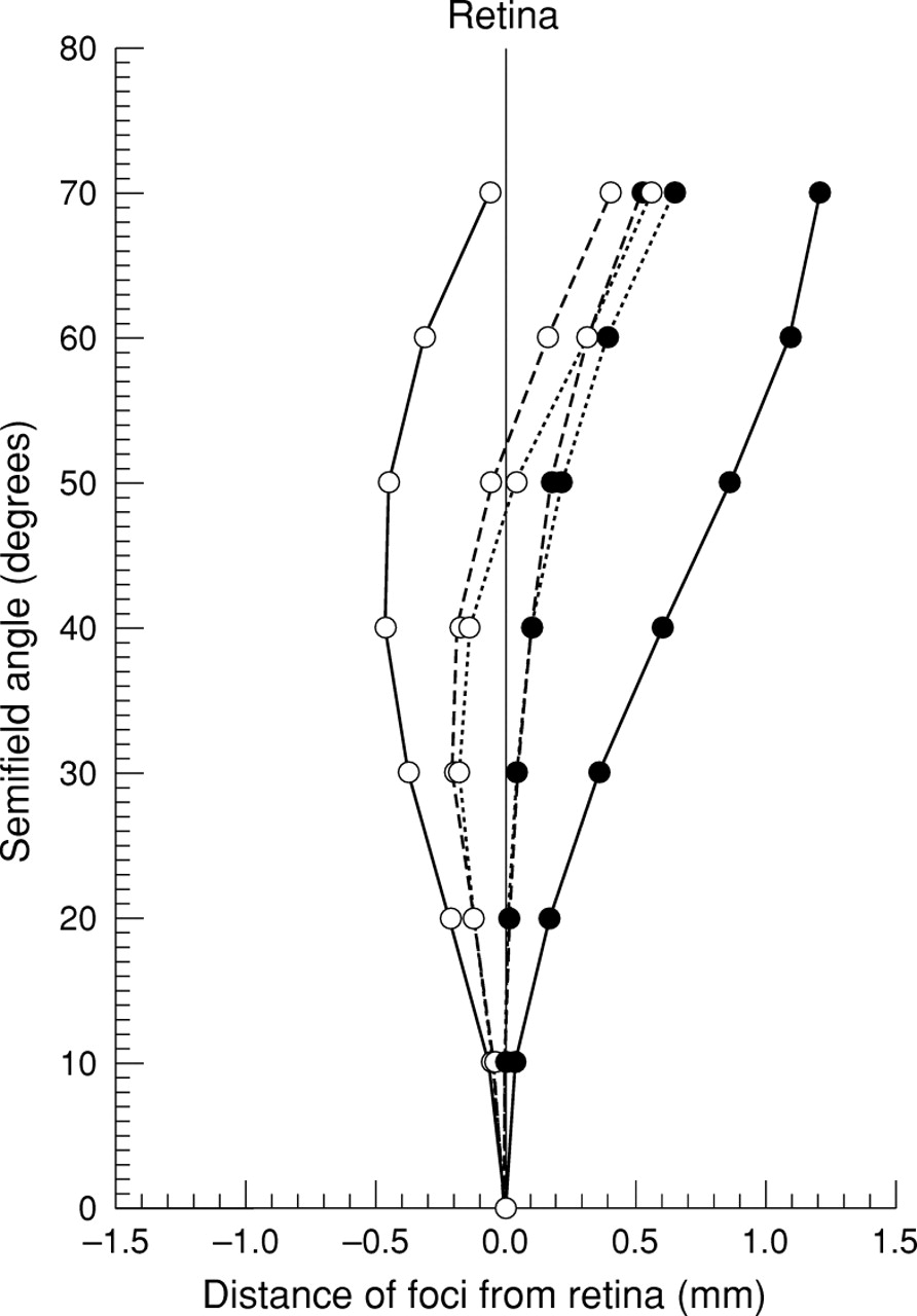
It is sometimes possible to change the shape of a lens to give stigmatic images as in point focal spectacle lenses. If this is achieved in the eye then both the sagittal and tangential image surfaces will lie on the retina. If this can not be achieved then the next best correction is to have the sagittal and tangential image surfaces equidistant from the retina such that the disc of least confusion lies on the retina. Figure 4 shows the sagittal and tangential astigmatic image surfaces for the Gullstrand–Le Grand schematic eye and also for single and double implant correction of the hypermetropic eye where the optimum lens shapes have been chosen (Table3). Two features are immediately apparent: firstly, the astigmatic difference is reduced for both pseudophakic eyes compared with the Gullstrand–Le Grand eye, and secondly, there is negligible difference between the astigmatism of a single implant lens and the polypseudophakic correction.

Sagittal (solid circles) and tangential (open circles) image surfaces plotted for the Gullstrand–Le Grand schematic eye (solid curves) and for the hypermetropic example eye corrected with both a single (broken curves) and double implant lenses (dotted curves). The disc of least confusion lies approximately mid way between the sagittal and tangential image surfaces.
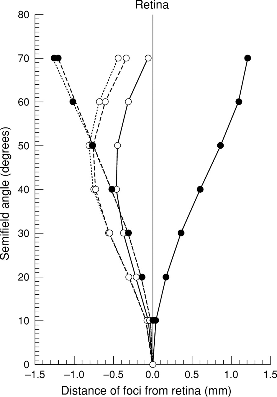
The specification of the nanophthalmic eye, taken from the biometry of Holladay et al 2 and specified in Table 1, does not allow astigmatism to be corrected since the plane of the front IOL was only 0.1 mm from the iris. Attempts to calculate the intraocular lens shape to correct oblique astigmatism with this location produce an unmanufacturable steep meniscus design. The implant lens(es) was therefore assumed to placed 1 mm behind the iris plane. The astigmatism curves of the nanophthalmic eye (Fig 5) also exhibit a significant reduction in the astigmatic interval compared with the Gullstrand–Le Grand eye. However, in both the hypermetropic and nanophthalmic eyes, for both single and double implants, the disc of least confusion, which lies approximately mid way between the tangential and sagittal foci, does not lie on the retina (this is a hypothetical vertical line on Figures 4 and 5 passing through x=0 mm). One of the reasons for this is that the retinal radius of curvature has been assumed to be −12.3 mm. This would be reasonable for an “average” eye but the radius of curvature is likely to be shorter for both our hypermetropic example eye and the nanophthalmic eye. We have not been able to find any data in the literature on retinal radius of curvature for strongly hypermetropic or nanophthalmic eyes. If the retinal radius of curvature was shorter, the effect would be to make the sagittal and tangential field curves more upright, helping to place the disc of least confusion closer to the retina. As a result, data on nanophthalmic and hypermetropic patients are likely to be better than our results shown in Figures 4 and 5 suggest.

Sagittal (solid circles) and tangential (open circles) image surfaces plotted for the nanophthalmic example eye corrected with both a single (solid curves) and double implant lenses (dotted curves). The disc of least confusion lies approximately mid way between the sagittal and tangential image surfaces.
Discussion
There is a significant improvement in the axial image quality measured in terms of MTF of the hypermetropic eye with double implants compared with a single intraocular lens implant (Fig 1). In terms of visual acuity, this improvement may not be clinically realised since both cases achieve theoretical Snellen ratios of 6/5 or better. An alternative and more practical way to look at these results is that the optical performance is better for the eye with double implants at low and mid spatial frequencies which are predominantly used in daily visual tasks. The better performance also allows a greater tolerance for manufacturing and positioning errors, as well as using readily available lens powers (theoretically both 21.1D). The results for the nanophthalmic eye (Fig 2) show a similar trend to the hypermetropic eye with a slightly poorer performance for the single implant lens (solid line in Fig 2), although both double and single implant corrections achieve 6/5 or better. However, such improvements here may be more academic since the vision in nanophthalmic eyes is often poor and it is less likely that patients would benefit from the improved performance. Even so, pragmatism would dictate that having two lenses 1 mm thick and with powers of 23.9D each is preferable to one IOL of power 47.8D which has to be at least 2 mm thick and where one surface has a radius of curvature a little over 4 mm.
Two further issues have been examined relating to axial image quality and possible optical limitations on maximum achievable visual acuity. Firstly, the optimum shape factors presented in Table 3 do not all conform to the commonly manufactured lens shapes which are equiconvex (B=0), biconvex (B∼0.6), convex-plano (B=+1) and plano-convex (B=-1). MTF curves were computed (not shown) for both the hypermetropic and nanophthalmic eye using the closest available commonly manufactured lens shapes. These were assumed to be either two convex-plano lenses (anterior surface convex for both lenses, B=+1) or two biconvex IOLs (most convex surface anterior for both lenses, B=+0.75). In both instances there was a negligible reduction in the MTF compared with the optimum designs. For the eyes studied we can conclude that it is not necessary to produce additional or customised lens shapes.
Secondly, Figure 6 demonstrates that correction of astigmatism using the optimum lens shapes given in Table 3 and illustrated in Figure 7can significantly reduce axial image quality. Plano-convex optics (posterior surface convex) are commonly used to help reduce posterior capsular opacification (PCO). If such lenses are potentially detrimental to axial image quality then a possible compromise is to consider using a plano-convex IOL for the posterior implant to help prevent PCO and then to use the lens shape which gives the best axial image quality for the anterior implant. Unfortunately this arrangement reduces the theoretical Snellen acuity from 6/3.6 (optimum for the hypermetropic eye, Fig 1) to 6/4.5 in the hypermetropic eye and from 6/4.4 (optimum for the nanophthalmic eye, Fig 2) to 6/5.3 in the nanophthalmic eye (MTF curves not shown). This reduction in estimated visual acuity is small and suggests that a clinical/optical compromise is possible.

Axial modulation transfer function (MTF) curves for double implant lens shapes that reduce oblique astigmatism (solid line) and which maximise axial image quality (broken line) implanted in the nanophthalmic example eye described in the text. The dotted curve represents the diffraction limit for a 4 mm pupil size with Stiles–Crawford correction and for a wavelength of 587.6 nm.

Single and double implant intraocular lens shapes that minimise oblique astigmatism. The lens shapes illustrated are for the hypermetropic eye described in the text. The intraocular lens shapes for the nanophthalmic eye are slightly more meniscus (see Table 3).
The results also demonstrate that the optimum lens shape for intraocular lenses, be they single or double implants, varies significantly between axial correction and off axis correction, in agreement with the findings of Atchison.23 25 Correction of primary astigmatism with lens shape can only be achieved if the IOL is placed away from the iris, assumed to be the aperture stop in all calculations. Even if the IOL is close to the iris then stop shift effects10 become small requiring extreme lens shapes to achieve the correction. The results in Table 3 demonstrate that concave meniscus lenses (shape factor B <−1) are required for single and polypseudophakic correction of primary astigmatism in the two example eyes. These lens shapes produce a significant reduction in the astigmatic difference (Sturm’s interval) over that of the modified Gullstrand–Le Grand schematic eye. It is possible that this could produce improved visual acuity across the field although there are several problems with interpretation. Firstly, it is necessary to know where the retina is in both of our example eyes. Data on retinal radius of curvature for the unusual eyes we are dealing with are not available to our best knowledge and so no qualified comment can be made as to the location of the disc of least confusion with respect to the retina. Secondly, there are other off axis aberrations which could reduce the performance, notably coma. However, the major drawback is that these lens shapes have significant axial spherical aberration. The estimated Snellen ratio falls in eyes with double implants corrected for astigmatism from 6/3.6 (optimum visual acuity) to 6/6.0 in the hypermetropic eye and from 6/4.4 (optimum visual acuity) to 6/20 in the nanophthalmic eye.
It would therefore seem unwise to use lenses corrected for oblique astigmatism since they decrease visual acuity. The only concreteoptical evidence against lenses that optimise axial image quality and hence acuity, is that computer ray tracing demonstrates that the spherical aberration corrected lens forms start to vignette at between 40 and 50° semifield angle. If visual field problems do present then it would be necessary to sacrifice some axial performance to improve the visual field.
All of the preceding analysis assumed idealised thin intraocular lenses. The validity of the thin lens approximation has been tested in two ways: firstly, the MTF curves were recomputed for thick lenses. This produced a negligible change in the MTF for the spherical aberration corrected lenses. However, thickening the lenses corrected for astigmatism has a more detrimental effect with the astigmatic interval increasing. In addition, the sagittal and tangential image surfaces are displaced posteriorly and hence the disc of least confusion lies further away from the retina (Fig 8). Secondly, a computer optimisation was used to see if our corrected lenses were optimum even when all aberration terms are considered and not just the primary aberrations. Again this made negligible difference to the spherical aberration corrected lenses. The conclusion is that the thin lens approximation is good for axial image quality but that astigmatism is much more sensitive to lens thickness.

Sagittal (open circles) and tangential image surfaces (solid circles) plotted for the nanophthalmic example eye corrected with thin double implant lenses optimised to give zero oblique astigmatism (solid curves). Thickening the lenses increases the oblique astigmatism and moves the image surfaces behind the retina (broken curves).
Finally, we note that higher refractive index materials—for example, acrylic, will always help to reduce monochromatic aberrations by reducing the surface curvatures. However, higher refractive index materials usually have a higher dispersion causing increased chromatic aberration that has not been considered here.
Conclusions
Double implants for extremely short eyes offer the potential for improved optical image quality. In this study the optimum lens shapes and power split between the lenses have been derived based on two example eyes and for both spherical aberration and oblique astigmatism. The level of improvement has been quantified using axial MTF curves for a 4 mm pupil size. Changes in the astigmatic image surfaces have also been studied. Results demonstrate that the improvement due to double implants may not necessarily manifest itself as improved acuity but almost certainly should benefit the majority of visual tasks that require low to mid spatial frequencies. These improvements can be achieved with currently manufactured lens shapes although using posteriorly convex IOLs to prevent posterior capsular opacification is likely to reduce the maximum achievable visual acuity.
Appendix
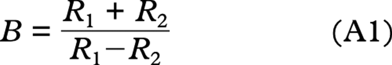
The lens shape factor is a dimensionless variable defined in terms of the curvatures R1 and R2 of the two lens surfaces and is given by10
The conjugate factor, defined in Welford,10 can be rewritten as

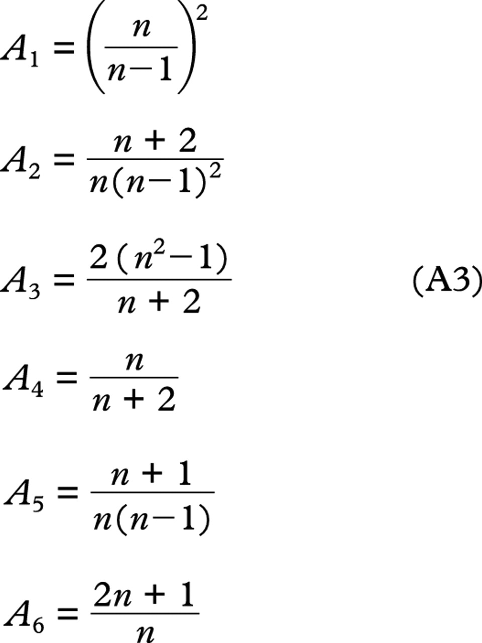
where L and L′ are the vergences just before and after the lens found by standard paraxial ray tracing through the system.25 Finally the coefficients Ai(n) are all functions of the reduced refractive index, n, defined as the ratio of the refractive index of the lens material to the index of the surrounding medium, no. The coefficients are defined by

For the calculations on spherical aberration, the procedure was as follows: firstly, the corneal power, IOL position, axial length, and refractive indices were specified. Standard vergence ray tracing techniques26 were then used to calculate the total power required for the IOL. If double implants were being considered then this power was divided equally between the lenses for the reasons given in “Methods”. The pupil radius was set based on the Stiles–Crawford adjusted pupil diameter suggested by Le Grand.20 A paraxial marginal ray, with a height at the cornea equal to the pupil radius and a slope angle of zero, was then traced through to the intraocular lens position using what is sometimes referred to generically as a “y-nu trace”.27 This gave the value for the ray height, h, needed in both equations (1) and (5). Once the conjugate factors had been calculated for the intraocular lenses present as indicated above, the primary spherical aberration can be found for any lens shape including that defined by equation (4) for minimum spherical aberration.
For the calculation of primary oblique astigmatism, both the Lagrange invariant, H, and the eccentricity variable E need to be calculated. The Lagrange invariant is given by
where β is the semifield angle, h is the pupil radius, and n the refractive index, which is 1 in this instance. The eccentricity variable, E is given by
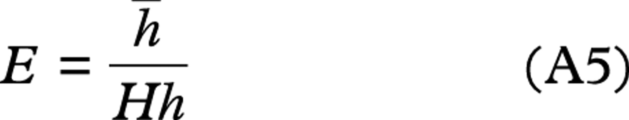
where− his the paraxial chief ray height and hthe paraxial marginal ray height both at the intraocular lens. Calculation of− his best achieved using commercial optical design software. This is because finding the chief ray requires a process called pupil exploration; the assumption that the chief ray passes through the centre of the iris (assumed to be the aperture stop) is not generally true when aberrations are present, as is the case here. Pupil exploration finds the exact values for the initial ray height and ray angle of the paraxial chief ray. Equation (5) can now be used to calculate astigmatism for any given lens shape.
The lens shape that produces zero astigmatism is found by setting equation (5) equal to zero. This results in a quadratic equation in B with the following coefficients:

which can be solved in the standard way. The lens shape chosen is the smallest one in magnitude. This helps to minimise the surface curvatures and makes the lens more manufacturable.