Article Text

Statistics from Altmetric.com
Modern cataract and refractive surgery aims not only to improve vision but to provide a good unaided visual acuity. Correcting astigmatic errors and control of surgically induced astigmatism are now an integral part of such operative procedures. Technological innovations and surgical developments in recent times have provided new methods for correction of astigmatism. However, evaluating the outcome of surgery for astigmatism presents particular difficulties, especially with the statistical comparison of different treatment groups.
In this review we will discuss the nature of astigmatism and its various refractive effects and how this relates to cataract and refractive surgical outcomes. The use and limitations of vectors and other methods for the analysis of change in astigmatism after surgery will be discussed along with appropriate statistical methods and suggestions for data presentation.
Ocular astigmatism
Astigmatism occurs when toricity of any of the refractive surfaces of the optical system produces two principal foci delimiting an area of intermediate focus called the conoid of Sturm. Thomas Young in 1801 was the first to describe ocular astigmatism, discovering that his own astigmatism was predominantly lenticular.1 However, it was some years later before Airy (1827) corrected astigmatism with a cylindrical lens.2 Corneal astigmatism was characterised by Knapp and also Donders in 1862 after the invention of the ophthalmometer by Helmholtz.34 In the same year Donders5 also described the astigmatism due to cataract surgery and soon after Snellen (1869) suggested that placing the incision on the steep axis would reduce the corneal astigmatism.6 Surgery to specifically treat astigmatism was suggested by Bates7 who described corneal wedge resection in 1894, but it was the work of Lans8 that provided most of the early theoretical basis for refractive corneal surgery. Little further work was published until that of Sato in the 1940s and 1950s.910 However, with the development of microsurgical techniques in the 1970s, Troutman once again popularised wedge resection and keratotomy for the reduction of astigmatism.1112
Why correct astigmatism?
Astigmatism induces distortion of the image.13-15When the effects of blurring of the image are excluded, the retinal image in an uncorrected astigmatic eye is distorted because of a differential magnification in the two principal meridians. Expressed as a percentage of the differences in these principal meridians (see equation 1 in the ), the image is distorted by about 0.3% per dioptre of astigmatism.14-16 In the corrected astigmatic eye, distortion of the sharp retinal image arises from the unequal spectacle magnification in the two principal meridians, which represents about 1.6% distortion per dioptre cylinder in the correction at the spectacle plane. This unequal magnification is manifest by altered shapes and by tilting of vertical lines (the declination error) that occurs maximally when the correcting cylinder is oblique (that is, 45° or 135°).13-21 Although oblique astigmatism only produces 0.4° of tilt per dioptre monocularly, it will produce major alterations in binocular perception.2
Despite the distortion induced by astigmatism, some astigmatism may be of benefit.141522-27 Various types of astigmatism have different effects on visual perception. For this reason the concepts of astigmatism “with the rule” (WTR) and “against the rule” (ATR) are clinically relevant. Astigmatism WTR is produced when the corneal curvature is steepest in the vertical meridian; conversely astigmatism ATR is produced when the steepest corneal meridian is horizontal.
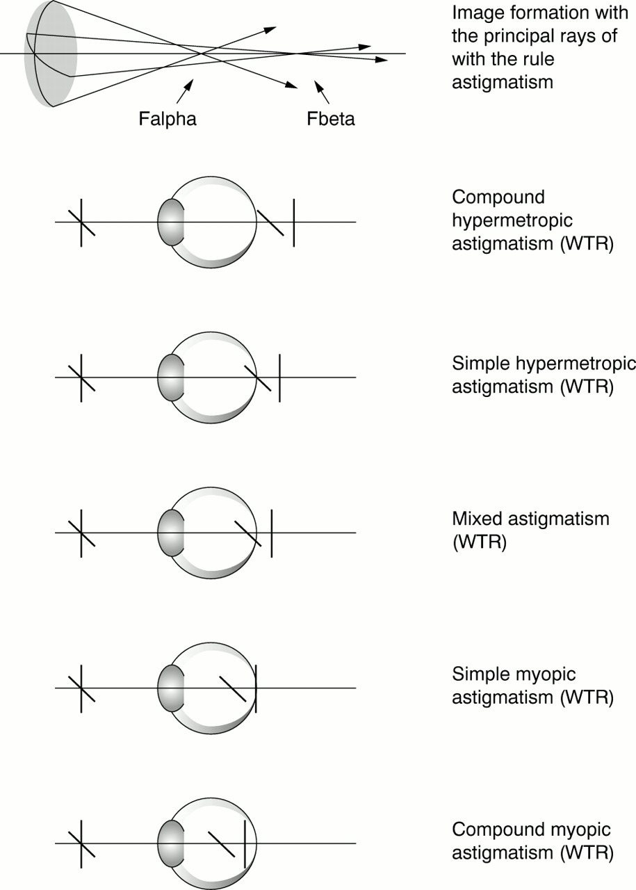
Figure 1 shows how the power of the weaker principal meridian produces a vertical line focus (Fbeta) in astigmatism WTR. In printed matter the vertical strokes of letters are more important for recognition—for example, b, d, h, t, p, y, also there is less space between letters on a line than between lines. In these circumstances it is most useful to have a better focus in the vertical meridian, as is produced by myopic astigmatism WTR resulting in better Snellen visual acuity than with ATR astigmatism.141528-30 Table 1 shows the effect of the orientation of the axis of astigmatism on Snellen visual acuity as described by Eggers.29 In addition, a number of psychophysiological responses are more sensitive to vertically oriented stimuli—for example, the stereoscopic threshold, the cyclodisparity range for fusion, and the monocular determination of depth using parallax errors.162021

Diagram showing the principal rays in the formation of an astigmatic image. Falpha is the anterior focal point, convergent light rays from the steeper meridian produce a horizontal line focus. Fbeta is the posterior focal point from the flatter meridian producing a vertical line focus. In this example, when Fbeta is coincident with the retina, simple myopic astigmatism with the rule is produced.
The approximate relation of unaided visual acuity and required correction (in dioptres) from 6000 refractions in young adults (males and females <30 years). The size of the plus cylinder for a given uncorrected astigmatic error was approximately 1.4 times greater than the spherical equivalent for an oblique axis, increasing to 1.6 times for a vertical axis (with the rule astigmatism) and 2.0 times for horizontal axis (against the rule astigmatism). The latter reducing to 1.8× when the VA was worse than 20/150. This demonstrates that against the rule astigmatism has a worse unaided VA and requires a larger cylinder correction than an equivalent with the rule astigmatism (that is, for any given spherical equivalent)29
Another little recognised advantage of astigmatism WTR is that less cylinder is required in the spectacle correction than for astigmatism ATR of the same magnitude.141531 This is known as Javal's rule (equation 2 in )32 and may partly explain the problem in only using keratometric data for the planning of refractive surgery described by some authors.3334
The reason for this relation is uncertain and could result from either lenticular astigmatism or a disproportionally shorter posterior corneal radius in the vertical meridian.31 Whether Javal's rule still holds after cataract extraction and intraocular lens implantation has not been determined; however, there is evidence that the spectacle cylinder correction is different from the keratometric astigmatism.21
Also, it is often not recognised that the spectacle cylinder will be less than the ocular astigmatism when the spherical equivalent (SEQ) is positive, and greater than the ocular astigmatism when SEQ is negative14313536 (equation 3). So in general, myopic ATR astigmatism will result in a proportionally larger spectacle correction, which of course will produce more distortion.
However, a certain degree of myopic astigmatism may be useful. Although never producing a crisp focus, this refraction may produce a situation of pseudoaccommodation in the pseudophakic patient.21-25This phenomenon was suggested originally in the 1960s by Peters,22 and by Huber.23 Later Sawusch and Guyton produced an elegant optical model indicating the optimal cylindrical component (C) for a given spherical equivalent (SEQ)26 (Fig 2, equation 4).

The ideal cylinder (C) for a given spherical equivalent (SEQ): C = −2SEQ − 0.50 (ie, C = −sphere − 0.25), where SEQ is −0.25 D or less (ie, a myopic correction) and C is a plus cylinder, and C = 2SEQ + 0.50, where SEQ is greater than −0.25 D (ie, a hypermetropic correction).26
Their model suggested that the least amount of summated blur throughout the range of object distances (0.5–6 metres) was −1.00 DS/+0.75 DC, and was closely followed by −0.75 DS/+0.50 DC.
Arguing that ATR astigmatism provides a superior uncorrected near visual acuity, Trindale et al discussed the astigmatic paradox.27 This is where the divergent rays from a near point are brought to focus more posteriorly by the fixed optics of the pseudophakic eye. So for myopic ATR astigmatism the vertical meridian will be placed closer to the retina for near objects, providing better visual acuity.
Apart from the bias of the psychophysical aspects of the visual perception towards vertically orientated objects, the physical optics of the eye also suggest that a small amount of astigmatism WTR is beneficial. This means that a relative value can be assigned to the various types of ocular astigmatism.
Astigmatism produced by surgery
Since Donders's first description, it was well recognised that the wound produced by cataract surgery produced astigmatism.5 Treutler described the outcome following superior section for cataract extraction for 49 patients in 1900.37 He found that the vertical curvature flattened by a mean of 0.7 mm (3.75D, up to 1.5 mm or 6.5D) for 88% of patients, for 2% there was no change, and for 10% there was an increase in curvature. With the advent of intraocular lens implantation and sutured cataract sections, induced astigmatism became more of a concern.35 Typically the tight sutures compressing the wound in the vertical meridian would produce an initial astigmatism WTR. Over a period of 3 months the astigmatism would change to ATR as the sutures loosened and the wound sagged with healing.38-42 The introduction of phacoemulsification of the lens nucleus and foldable intraocular lenses resulted in smaller wound producing less astigmatism.43-46 Placement of the wound on the horizontal corneal meridian has become more common and results in less change in the astigmatism as the wound heals.47-49 Although the use of different suture materials, suturing techniques, and other suture manipulations may influence the early postoperative outcome, the ultimate astigmatic result is predominately influenced by wound size and placement.4050-55
During the evolution of change in astigmatism following cataract surgery, the patient's actual spherical equivalent will remain constant. Cravy described this effect as being not unlike a “hula hoop” where compression in one axis results in an equal expansion in the other axis.56 He was in fact describing Gauss's law of elastic domes—“for every change in curvature in one meridian there is an equal and opposite change 90° away.” This phenomenon of corneal behaviour is known as the coupling effect.85758 Thornton restates Gauss's law as “the law of modified living elastic domes—the change in the primary meridian is proportional to the change in the primary meridian reduced by the increase in circumference.”57 Therefore the corneal curvature changes are not as if a single spherocylinder was placed at a certain axis, but as if a plus cylinder was placed in the steeper meridian and a minus cylinder of equivalent magnitude was placed in the flatter meridian (that is, a cross cylinder effect). The concept of a cross cylinder effect is an important consideration in the method of analysis of astigmatic changes.
Coupling also occurs with tangentially oriented corneal incisions and is predictable enough to form the basis for astigmatic keratotomy.57-60 Placing an incision perpendicular to the steepest corneal meridian in the mid-periphery of the cornea will flatten the curvature in that meridian as a result of wound gape. It will also result in the steepening of the flatter corneal meridian because the boundary of the cornea is fixed by the limbus. In general, the plus cylinder notation is used because the incisions are placed on the cornea straddling the axis of the plus cylinder.5859
Laser photorefractive keratectomy also has the ability to correct the corneal astigmatism at the same time as correct myopia.6162 In effect the procedure cuts a minus cylinder from the corneal surface, so minus cylinder notation is usually used. For the correction of hypermetropic astigmatism a plus cylinder notation is used to minimise redundant ablation. The result produced is independent of the coupling phenomenon and is only influenced by the healing response of the patient changing the profile of the ablation over time.
Misalignment of the wound will result in a residual error of refraction in all types of refractive surgery. As a corrective cylinder is rotated away from its correct axis without a change in its magnitude, residual astigmatism is induced. The effect of cylinder misalignment is essentially the same as that of obliquely crossed cylinders.14-163163 For example a −1.00 D cylinder rotated 10° off an intended axis of 180° will result in an error of +0.17/−0.35 × 140° (see equation 5). A general rule of thumb for this circumstance is that the magnitude of the cylindrical error is 3.5% of C per degree of φ and lies about 45° from the axis of C.64 This relation explains the need to adjust the sphere with any change in the cylinder power or axis during refraction. The fact that the components of the refraction are not independent of one another presents difficulties with the analysis of change in refraction, as is discussed later.
So as the axis of the cylindrical correction is rotated away from its correct position the power of the cylinder needs to be reduced in order to minimise the residual astigmatism (Fig 3, equations 5, 6, and 7).1665-68

Residual astigmatism produced when a cylinder axis is shifted away from its correct position: (Csinφ) DS/−2Csinφ) DC, axis (θ + 45 + φ/2), where C cylinder is set at φ angle from the true axis θ. Graphs illustrate how reducing the cylinder power to an “optimal value” can minimise the residual astigmatism. The optimal cylinder power in these circumstances is: Ccos2φ, where C is the original full dioptric power of the correcting cylinder, and φ is the angle the cylinder is rotated away from the correct position. So if the “optimal value” for the correct cylinder power is used the residual astigmatism is equal to Csin2φ, where C is the original full dioptric power of the correcting cylinder and φ is the angle the cylinder is rotated away from the correct position.16
When evaluating the effect of the refractive surgery, the surgeon wishes to know what the patient's refractive result means in terms of surgical error. That is, was the error in the magnitude of the surgical correction (resulting in astigmatism of −2Csinφ), and what was the error in axis alignment (φ) of the correction which, as discussed, has a direct influence on the magnitude error. Many of the methods of analysis suggested for this purpose follow.
Vector analysis of surgery of astigmatism
Much has been written about the vector analysis of astigmatism.814333869-84 For the average ophthalmologist the concept is rarely used in clinical practice because of the daunting trigonometry involved, producing a result which seems remote from the refraction actually presented by the patient.
The basis for all the methods of vector analysis is the theory of obliquely crossed cylinders originally described by Stokes.63 Naylor suggested that the formula could be used to determine the difference in refraction brought about by surgery.69
The principle assumes that a theoretical spherocylinder, the surgical induced astigmatism (SIA or CSURG × β°) is “crossed” with the preoperative refraction to produce the postoperative refraction (Fig 4, equation 8).
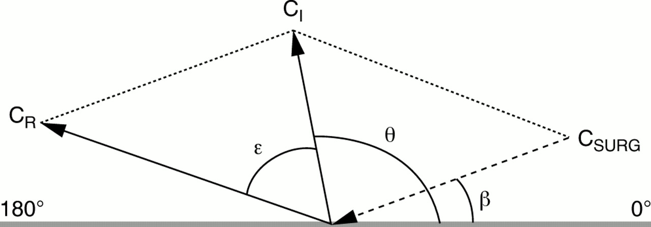
Diagram demonstrating the principle of vector analysis of the change in the astigmatic refraction following surgery. The arrow direction represents the axis of astigmatism and the length the magnitude. The principle assumes that a theoretical spherocylinder, the surgical induced astigmatism (SIA or CSURG × β°) is “crossed” with the preoperative refraction to produce the postoperative refraction69: SI/CI× θ° + SSURG/CSURG × β° = SR/CR × (θ + ε)°, CSURG = (CI2 + CR2 − 2 CI CR cos2ε), SCYL = (CI + CSURG −C R)/2, sin2β = (CR/CSURG) sin2ε, SSURG = SR − SI − SCYL; CIis the initial or preoperative astigmatism vector at θ° axis (in “plus” cylinder notation), CR is the resultant or postoperative astigmatism vector at θ + ε° axis (“plus” cylinder notation), CSURG is the surgically induced astigmatism vector (SIA, a theoretical construct) at β° axis (in “minus” cylinder notation), SCYL is the spherical equivalent of all the cylindrical components.
Figure 4 shows the graphical solution for the resultant of two obliquely crossed cylinders where the SIA equals the initial refraction minus the final refraction.
The “law of cosines” was further promoted by Jaffe and Clayman38 and has resulted in a many subsequent publications about methods of calculation of the SIA.1433384569-84 The main problem encountered is that the standard axis notation for cylinders (Axint, adopted at the 1950 International Federation of Ophthalmic Societies) only ranges from 0 to 180°. The formula as you can see addresses this by doubling the angle of astigmatism, but care is required when using the tangent function to determine the axis of the SIA and needs an understanding of when a 180° correction is required.
On its own the SIA vector does not reflect the actual refractive outcome in any tangible way for the patient and surgeon alike. The reduction of astigmatism, which is a spatial entity that has curvatures in more than one plane, into a unidirectional arrow on a polar plot not only results in the loss of data but also introduces its own distortion of reality.85 This is because the SIA vector is only a theoretical construct and has no structural existence. Vector analysis alone does not provide any indication of the relative value of the surgical procedure. The magnitude and orientation of astigmatism WTR or ATR is better described by the actual refraction or keratometry of the patient.
Vector analysis is a mathematically correct method of describing the relation between the initial and resultant cylinder. It provides information about the process by which the surgical outcome (the resultant cylinder) was achieved. However, for the surgeon in particular, the surgical vector alone does not really provide practical information about the surgical error. To be useful the surgical vector requires further translation.
Optical decomposition of the cylinder
Although Gartner86 from Australia was the first to describe the principle of optical decomposition of the cylinder, Humphrey recognised and capitalised on its utility before others. Humphrey's work has only recently been described in the ophthalmic literature although the principle of astigmatic decomposition was an innovative part of the Humphrey vision analyser patented in 1977.8788 Humphrey stated that any spherocylinder may be expressed as the mean refractive error (that is, the spherical equivalent) in conjunction with two cross cylinders fixed at 0,90° (J0) and at 45,135° (J45). This can be achieved as follows1688:
SEQ = S + C/2
J0 = C × cos2θ
J45 = C × sin2θ
where S is the spherical power and C is the cylinder power at θ° axis.
Faced with the problem of analysing simultaneous changes in both direction and magnitude of astigmatism and acknowledging that vector analysis alone was not particularly useful, Cravy also suggested a method of astigmatism analysis that used optical decomposition of the astigmatism (apparently independently of Gartner's and Humphrey's work).56
Cravy reduced the keratometric astigmatism into an x or ATR and y or WTR component (equation 11, Fig 5).

Diagram demonstrating the principle of decomposition of the astigmatic refraction into x and y values. Cravy56suggested that cylinder (or astigmatism) of M magnitude at θ° axis maybe characterised by a “y” magnitude at 90° axis (y = M sin θ) and an “x” magnitude at the 0–180° axis (x = M cos θ). Naeser described a single summary value for the astigmatism which he called the polar value of net astigmatism (KP).82838589-91 This was originally calculated as89: KP = M × (∣sin θ∣ −∣cos θ∣), but modified later to90: KP = M × (sin2 θ − cos2 θ), where M is the magnitude and θ is the axis of astigmatism, and KP is the polar value referable to the 90° meridian (ie, encompassing the WTR and ATR concept). When sin θ > cos θ, (ie, y > x), the more WTR the astigmatism and the more positive the polar value. Conversely when sin θ < cos θ (ie, y < x) the more ATR the astigmatism and the more negative the polar value.
x = M × cos θ
y = M × sin θ
where M is the magnitude of astigmatism and θ° is the axis of astigmatism.
He then used these polar coordinates to derive a unitary number (ΔK) that described the astigmatism in terms of a WTR or ATR change. This required assigning a plus or minus to the polar value depending upon the change in the x or y value as a result of the surgery. Although this method assigned a relative value to the astigmatism, it was awkward to program for computers and only referred to a change in the astigmatism (ΔK).
Taking the concept of optical decomposition further, Naeser was able to demonstrate a simple mathematical relation that assigned a relative value to the astigmatism. He called this value the polar value of net astigmatism (KP).82838589-91
The KP value was described a number of ways previously (equation 12), but more recently Naeser further modified this formula to calculate the polar value referable to the surgical plane (that is, the meridian on the cornea where the surgical wound was placed or aligned). So changes in the astigmatism projected on the steeper meridian are called “with the power” (WTP) and “against the power” (ATP) when projected onto the flatter meridian (rather than just to the 90° degree meridian as before)85:
AKP = M × (sin2[α + 90] −β) + cos2([α + 90] −β)
where M is the magnitude of astigmatism, α is the powermeridian of net astigmatism (that is, α + 90 is the axis of astigmatism), and β is the direction of the surgical plane (that is, the axis about which the surgical wound was placed), so AKP is the astigmatic polar value of net astigmatism.
So when the wound is placed at the 12 o'clock position the result is as before. To examine the WTR/ATR relation β is denoted as 90° regardless of the surgical plane.
In the analysis of a surgical result the polar value change “on” the surgical axis will provide an index of the efficacy, and the “off” the surgical axis astigmatism (that is, the net corneal astigmatism) an index of the accuracy of the refractive surgery.
Kaye et al suggested that a simple measure that reflects the surgical accuracy (SA) of a procedure could be expressed as the ratio of the “effectiveness” of the SIA vector to the sum of the SIA and resultant astigmatism (CR).78 The “effectiveness” of the SIA (′CSURG) was defined as the net effect of the SIA vector at 90° to the initial astigmatism (CI). This was calculated by subtracting the decomposition of the SIA vector to an axis at 90° from the initial astigmatism (equation 14, Fig 3). The maximum SA will be 1.0 when ′CSURG equals CSURG thus CR is zero. Any axis misalignment or magnitude error would produce an SA of less than 1.0; however, the relative contribution of either of these two errors would not be distinguishable.
Olsen and Dam-Johansen described how the surgical vector between the initial and resultant cylinder vectors could be optically decomposed into the WTR and WTR meridians (similar to the Cravy method).84 This was to allow for the simultaneous presentation of magnitude and direction over time. Although Olsen's method highlights the need to translate the surgical vector into something meaningful and provides a relative value to the results of vector analysis, it still only describes the process rather than the outcome of the surgery. The translation fails to provide the necessary information about the surgical error of the procedure for the individual patient.
In an elegant synthesis of optical decomposition methods, Naeser and Behrens recently demonstrated that the calculation of two polar values 45° apart where equivalent to Humphrey's Jo and J45 (equation 15).83
KP(90) = M × cos2θ = J0
and
KP(135) = M × sin2θ = J45
Naeser and Behrens then showed that there is a nexus between polar values and vector analysis. After determining the KP(90) and KP(135) values for the preoperative (CI) and postoperative (CR) astigmatism the SIA is simply calculated as:
SIA KP(90) = CI KP(90) − CR KP(90)
and
SIA KP(135) = CI KP(135) − CR KP(135)
where SIA is the surgically induced astigmatism, CI = the initial cylinder, and CR = the resultant cylinder (the magnitude and direction of the SIA vector can be found using the Humphrey notation re-conversion formulas, equation 10).
Using a different approach, Thibos et alalso demonstrated the nexus between methods of optical decomposition of the cylinder and vector analysis.92 They describe the spherocylinder using Fourier analysis of the power profile of the refractive surface. Fourier analysis transposes a complex waveform into a constant and harmonically related sine and cosine waves—the constant being the spherical lens power, and the harmonic being the pure cylinder power (equation 17).
In fact the cylinder power represents a Jackson cross cylinder where the mean spherical equivalent is zero, and the cylinder power J = C/2. Raasch describes the transformation of the spherocylinder power as a sum of 3 component terms—the spherical equivalent (SEQ = S + J), cosine astigmatism (Cs, the WTR/ATR component) and sine astigmatism (Sn, the oblique astigmatism) (equation 18, Fig 6) so that93:

Diagram of the Fourier decomposition of a spherocylindrical lens (S = plano/C = −3.25 × θ = 70). The 360° lens surface power (ie, for all meridians) is represented by the thick line. The three Fourier component terms are: a spherical equivalent (SEQ = S + C/2), a cosine astigmatism term (J × cos2θ), and sine astigmatism term (J × sin2θ) where J = C/2.93
where P is spherocylindrical power, S the power of the sphere, J half the cylinder power (C), and θ the axis of C.
The similarities of the Fourier transform to the Naeser formulas for KP(90) and KP(135), and the Gartner/Humphrey method of decomposition are apparent. Fourier transformation also provides a nexus with the power matrix method of astigmatism analysis previously described (equation 19).7475
The use of Fourier analysis extends beyond simple astigmatism. Raasch and others have demonstrated that Fourier analysis transforms the complex representations of corneal curvature produced by corneal topographic analysers from videokeratographs.94-98 With this method the topographic data are reduced to spherical equivalent power, and harmonics of decentration (first), regular astigmatism (second), and irregular astigmatism (third or higher order). This not only provides a powerful method of astigmatism analysis of complex data, but also a reliable method of data compression.
By using two polar values or the sin/cos Fourier values the astigmatism may be more completely characterised. For example, calculating a polar value in the plane of the incision will indicate the magnitude effect of the surgery—a positive value indicates steepening of the surgical meridian a negative value indicates flattening. Calculating another polar value at 45° to the surgical plane will indicate the degree of cylinder rotation induced by the surgery—the larger the value, the greater the rotation with a zero value indicating no rotation.
Optical decomposition methods are attractive because the cylinder (expressed as magnitude and direction) is translated into two standard reference points (two magnitudes). Naeser's method in particular demonstrated that these methods can produce a relative value consistent with the WTR/ATR concept. Assigning a relative value enables one to make a meaningful comparison of the astigmatic outcomes between groups of patients.
Other methods of analysis of the astigmatic effect of surgery
The final result of refractive surgery may be influenced by the healing response, but the initial refractive outcome is determined by the accuracy of the axis alignment, and the quantity of change induced by the surgical procedure. Although both the components of the surgical error are interdependent, any axis misalignment will produce a magnitude effect of its own which, as previously discussed, will be proportional to the magnitude of cylindrical power produced by the surgical manoeuvre. To assess the effect of the procedure the surgeon would wish to know the error in achieving the target astigmatism—that is, was the axis placement correct and the quantity of the procedure enough?
The general aim of refractive surgery is to reduce the astigmatism. Conceptually it is easiest to consider the astigmatism in “plus cylinder” notation, so that the surgery then acts as if adding a “minus cylinder.” When expressed as vectors, the surgical cylinder arrow would point in the opposite direction to the initial cylinder arrow. Vector analysis can now be usefully employed using this concept because the surgical error can be determined by the simple subtraction of the surgical vector from the initial cylinder vector.34This will provide the magnitude (CERROR) and angle (φ) error of the surgery (equation 20, Fig 7).

Diagram demonstrating the use of the vector representation of the astigmatic refraction to determine the quantities of surgical error. The magnitude error (CERROR) is the simple subtraction of the absolute CSURG magnitude from the absolute CI magnitude in dioptres cylinder. The direction or axis error (φ) is the CSURG axis (β) in minus cylinder notation from the CI axis (θ) in plus cylinder notation.34
Alpins also introduced the concept of “target induced astigmatism” (TIA), highlighting the concept of a planned astigmatic outcome as an integral part of modern cataract and refractive surgery.33TIA was described as the cylinder vector of the desired change intended by the surgery, enabling the surgeon to match it with the SIA to determine the success or otherwise of the surgery. The surgical error can also be determined with regard to the planned resultant cylinder, the TIA (or planned) vector is subtracted from the surgical vector.
The concept of the surgical error of a procedure calculated from the vector analysis provides the surgeon with practical data to understand how the surgical process has produced the resultant cylinder. This of course is only valid in the early postoperative period before the healing response has modified the initial result of the surgery.
Statistical analysis of astigmatic changes after surgery
Lack of critical evaluation of the utilisation of the surgical vector has resulted in its adoption as the de facto standard used in most reports concerning the surgical management of astigmatism.9199-103 Rather than describing an outcome, vector analysis best describes the process producing the surgical outcome. As a process measure it is only a conceptualisation relevant to the individual patient and not particularly useful as a population statistic, largely because it does not assign a value to the outcome. Moreover, Toulemont demonstrated that the formulas used to calculate the vectors are non-linear and introduce errors when using standard statistical analysis.76
Process measures relate to the events that produce an outcome. Accuracy is generally indicated by the mean effect produced by the event, whereas precision is indicated by the spread of the means (the standard error). However, the actual outcome (for example, the manifest postoperative refraction) is a more meaningful way to interpret the effect of a surgical procedure in population terms, particularly when comparing a number of different processes attempting to produce the same desired result. None the less, a meaningful result can only be found if a relative value is assigned to each outcome.
Serial measurements present particular difficulties in analysis.104 If chosen incorrectly the statistical the analysis often fails to answer clinically relevant questions. The use of the change in vector analysis over time is conceptually invalid, because the unlike the initial surgical event, the wound healing process is continuous. Mathews et al argue that the commonly used comparison method of a series oft tests at each time point is flawed for three main reasons.104 The first is that the curve joining the means may not be a good descriptor of a typical curve for an individual. Secondly, the analysis does not take account of the fact that measurements at different time points are from the same subjects so are not independent measures and, lastly, successive observations on a given subject are likely to be correlated. They suggest that a more appropriate method is to choose a suitable summary of the response of an individual then analyse these summary measures as if they were raw data using simple statistical techniques. However, choosing one or more clinically appropriate summary measures from a time series requires care.
Summary measures such as the peak postoperative astigmatism, the final stabilised postoperative astigmatism (along with the proportion of WTR versus ATR), and the rate of change in the postoperative astigmatism would be appropriate for post-cataract surgery. The time to achieve a stable refraction would also be appropriate if sufficient measurements are made over the critical time period. For refractive surgery, such as arcuate keratotomy and excimer laser PRK outcome measures such as the surgical error (degree of axis misalignment and undercorrection or overcorrection of the cylinder magnitude) would be appropriate, as would the final stabilised postoperative refraction.
Even once the appropriate summary measure has been determined, the analysis of refractive changes is further compounded by the fact that the refraction consists of the sphere, cylinder and axis—all of which may change with time. For this reason optical decomposition methods are useful summary measures. Not only do they reduce the astigmatism from magnitude and direction down to two magnitudes it is also possible to assign a relative value to produce one summary value.
Bennett and Rabbetts suggested that the optical decomposition method of Humphrey was an appropriate method to determine the mean of any number of refractions,14 which was also the basis of Olsen's method84 and Naeser's most recent method.8391 Each one of the three components could be separately summed, and the individual refractions first separated into groups of WTR or ATR if necessary. Cravy's and Naeser's approaches produced a single polar value to characterise the astigmatism and Kayeet al also demonstrated a method of producing a single summary value.567883858990Although each is an elegant compromise, these methods compress the data and are insensitive to oblique astigmatism. Polar values may be appropriate summary measures but they are inappropriate for sequential analysis at individual time points for the reasons already outlined.
However, the problem with all simple analysis is the difficulty in producing a standard deviation for a number of refractions because separate analysis of each component is statistically invalid.104 The statistical methods must make full and joint allowance for all the components of the refraction and may be best achieved by the use of multivariate methods of statistical analysis. Generally, three approaches to the problem have been described. For the cylinder power and axis alone others have used the Hoteling T2 statistic,105 or bivariate probabilistic analysis.77 For sphere and cylinder refractions Harris suggests converting the refraction to a power matrix and using his w statistic and F distribution to compare the groups.106107 Note, however, a relative value is not assigned using any of these methods.
Most methods suggested by others double the axis of astigmatism for analysis so that the ATR astigmatism values that are separated with the standard axis notation are brought together by the 360° polar transformation. Another method of addressing the problem of the split ATR astigmatism values is to transform those values above 90° into “mirror equivalent” values less than 90°. Converting to mirror equivalent values bring the ATR values together, but unlike the double angle method, the oblique astigmatism values are also brought together so that all the values are conveniently presented in one quadrant (see Fig 8C and Table 2). For example, an angle of 175° would convert to 5°, 135° to 45°, and 100° to 80°. Although this results in some data compression, it is clinically relevant and totally in keeping with the concept of astigmatism orientation. Not only does it allow a relative value for grouped data to be assigned at a glance, it greatly improves the method by which data can be presented.

Methods of presenting astigmatism data. The same base data set is used for all the methods of presentation shown in Figures8, 9, and 10. The data are from two groups of patients who had extracapsular cataract surgery. (A) The change in mean magnitude of astigmatism. (B) The change in the mean Naeser polar value (positive values are with the rule, negative values against the rule). (C) The change in the “expectancy” of astigmatism from 1 week postoperative (no 1) to 12 months postoperatively (no 8) using the “by the rule” or mirror equivalent axis conversion. The “expectancy” is a statistically correct bivariate (or simultaneous) calculation of the magnitude and axis for the grouped astigmatism data (as opposed to the incorrect method of calculating the simple mean of the magnitude or axis independently). This was calculated using the contingency table method of Toulemont.78 The axis values were first converted to mirror equivalent values as shown in Table 2.
Transforming the astigmatism from 0–180 (Axint cylinder notation) to 0/180–90 (“by the rule” notation, ie, mirror equivalents). This allows the ATR and oblique astigmatism values to be grouped together. This may be computed with an if, then, else statement—eg, if θ > 90, then ′θ = 180 − θ, else ′θ = θ
Optical decomposition consistent with the Fourier analysis methodology is possible using the “by the rule” transformation of the cylinder axis:
′Sn = J × sin(′θ)
′Cs = J × cos(′θ)
where J = C/2, half the cylinder power and ′θ is the “by the rule” or mirror equivalent axis.
For the whole refraction:
′P = [S + J − ′Cs − ′Sn]
where S + J = SEQ the spherical equivalent, and for the astigmatism power alone:
′Pa = [J − ′Cs − ′Sn]
where ′Pa is the “by the rule” transformed astigmatism power.
Although ′Pa may be a used as a summary measure, it does not produce a linear progression and deals with the problem of oblique astigmatism poorly. As can be seen in Table 3 not only are the values for the WTR and ATR axes equivalent, the more oblique values better weighted.
Examples of astigmatism power (′Pa) calculated for various “by the rule” axis values of J astigmatism from 1.00 to 5.00 D
The “by the rule” cosine astigmatism (′Cs) shown in Table 4 is also an inadequate summary measure. Although ′Cs increased for the magnitude of astigmatism as the axis changes from WTR to ATR, the progression is non-linear and all the 90° values are null.
Examples of cosine astigmatism (′Cs) calculated for various “by the rule” axis values of J astigmatism from 1.00 to 5.00 D
To produce a linear progression in which a single individual value for each astigmatism a simple rank could be assigned using the “by the rule” axis of astigmatism such that:
R = M − (′θ/400)
where M is the magnitude of astigmatism and ′θ the “by the rule” axis.
Although this method of ranking the astigmatism assigns a better value to the oblique astigmatism than the ATR astigmatism, R is easily computed by a spreadsheet. The effect of the SEQ (equation 3) may also be computed by a spreadsheet to transform R to further delineate its relative value as part of the whole refraction.
Another method that may better encapsulate a relative value is by manually assigning a score to each patient's refraction or astigmatism. This method assumes that a lower magnitude of astigmatism WTR is most desirable and that a higher magnitude oblique astigmatism is the least desirable outcome (Table5).
An example of manually scoring the astigmatism to produce a summary measure for statistical analysis. The actual steps in the magnitude may be altered to suit the clinical situation requiring analysis. Smaller increments maybe suitable when larger numbers of patients are involved
The data generated by this scoring methods may be regarded as ordinal categorical (or continuous) data, amenable to analysis by a large number of well established statistical procedures, including multiple linear or logistic regression. Another advantage is that for any pair of scores, the higher is always clinically interpretable as the least desirable. This is not the case for most other methods.
Data presentation
Many of the aforementioned papers and others have suggested methods to present the data after cataract surgery.72 Like the problem with the analysis, displaying the concurrent change in magnitude and axis of astigmatism over time presents difficulties. A series of 360° polar scatter plots may produce an overview of the spread of the data but poorly presents the mean data and separates the oblique astigmatisms.105 A plot of the magnitude of astigmatism alone is useful because this is the major component determining the quality of the refractive outcome (Fig 8A). The effect of the direction of the astigmatism combined with the magnitude over time may be demonstrated with plots of polar values (Fig 8B). More succinct graphs such as Figure 8C which use mirror equivalent values compress the data into one quadrant with each point representing the mean value at a particular time. Another method is to use balloon plots (Fig 9), the position relates to the direction and the size to the magnitude of the astigmatism—these can be plotted along a time line as is the convention. Frequently, histograms are a good way of comparing the summary measures (Fig 10). The magnitude and direction can be compared independently; alternatively a contingency table may be put into a three dimensional density plot.77 The surgical error is also conveniently plotted as a histogram for magnitude and cylinder error.
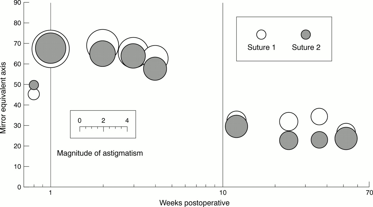
Methods of presenting astigmatism data. The same base data set is used for all the methods of presentation shown in figures8, 9, and 10. The data are from two groups of patients who had extracapsular cataract surgery. The change in the “expectancy” of astigmatism regraphed as a balloon plot.

Methods of presenting astigmatism data. The same base data set is used for all the methods of presentation shown in figures8, 9, and 10. The data are from two groups of patients who had extracapsular cataract surgery. The change in magnitude and axis (converted to mirror equivalent values) of astigmatism and Naeser polar values plotted as frequency histograms at 1 week and 3 months postoperatively.
Conclusion
The astigmatic results of refractive surgery are best evaluated in terms of a relative value. In general, any residual astigmatism is best when “with the rule” and worst when oblique; however, the magnitude of the astigmatism is the predominant concern.
Vector analysis provides information about theprocess of the surgery and is most useful when translated into quantities of surgical error. However, the effect of wound healing is continuous and inappropriately summarised by vector analysis, which does not give a measure of outcome.
Because of the different effects of “with the rule” and “against the rule” astigmatism on vision, when comparing different groups or methods, the outcome is best evaluated using a summary measure that assigns a relative value to the result such as Naeser's or Cravy's method. However, neither of these methods adequately assesses obliquity of astigmatism.
Better evaluation of the effect of astigmatism axis requires the use of the “by the rule” or mirror equivalent axis notation, or by a manual scoring method to produce an outcome summary measure.
Thus, different methods of analysis are available to study the effect of surgery on astigmatism, several may be required to summarise both process and outcome.
Acknowledgments
Our thanks to Peter Lindsay, Bill Aylward, Julian Stevens, and Geoff Woodward for helpful discussions during the preparation of this paper. Data for Figures 8, 9, and 10 were from a study funded by Davis and Geck. Our thanks to those authors who kindly provided reprints of their articles.
Appendix
Equations:
(1) The percentage distortion of anastigmatic lens14:
100 × (dα − dβ)/dβ
where dα is the dioptric power of the first principal focus of an astigmatic image and dβ is the dioptric power of the second principal focus.
C = 1.25M − 0.50
where C is the cylindrical power in the spectacle correction and M is the magnitude of corneal astigmatism, which is regarded as positive with the rule (WTR) and negative against the rule (ATR).
(3) Spectacle cylinder power14313536:
C ≈ (1 − 2dSEQ) M
where d is the vertex distance of the correcting cylinder C, SEQ is the spherical equivalent and M is the magnitude of corneal astigmatism.
(4) The ideal cylinder for a given spherical equivalent25:
C = −2SEQ − 0.50 (ie, C = − sphere − 0.25)
where SEQ is −0.25 D or less (ie, a myopic correction) and C is a plus cylinder, and
C = 2SEQ + 0.50
where SEQ is greater than −0.25 D (ie, a hypermetropic correction).
(5) The effect of misalignment of a correcting cylinder—that is, the combined cylinder power and axis produced by two obliquely crossed cylinders1665-68:
(Csinφ) DS/−2Csinφ) DC, axis (θ + 45 + φ/2)
where C the correcting cylinder is set at φ angle from the true axis θ, DS = resultant sphere (dioptres), DC = resultant cylinder (cylinder).
(6) The optimal cylinder power to minimise the residual astigmatism from axis misalignment of a correcting cylinder1665-68:
Ccos2φ
where C is the original full dioptric power of the correcting cylinder and φ is the angle the cylinder is rotated away from the correct position.
(7) If the “optimal value” for the correct cylinder power is used, the residual astigmatism is:
Csin2φ
where C is the original full dioptric power of the correcting cylinder and φ is the angle the cylinder is rotated away from the correct position.
(8) The theoretical “astigmatic correction” of surgery—the surgical induced astigmatism (SIA or CSURG) is calculated by subtracting the initial refraction from the resultant refraction69:
SI/CI × θ° + SSURG/CSURG × β° = SR/CR × (θ + ε)°
CSURG = (CI2 + CR2 −2 CI CR cos2ε)
SCYL = (CI + CSURG − CR)/2
sin2β = (CR/CSURG) sin2ε
SSURG = SR − SI − SCYL
where SI and CI at θ° axis (in “plus” cylinder notation) is the initial refraction, SR and CR at θ + ε° axis (“plus” cylinder notation) is the resultant refraction, and SSURGand CSURG at β° axis (in “minus” cylinder notation) is the difference in the refraction brought about by surgery, otherwise known as the surgically induced astigmatism SIA (SCYL is the spherical equivalent of all the cylindrical components).
(9) The optical decomposition of a spherocylinder into a spherical equivalent and a cross cylinder fixed at 0,90° (J0) and at 45,135° (J45) (“Humphrey” notation)1688:
SEQ = S + C/2
J0 = C cos 2θ
J45 = C sin 2θ
where S is the spherical power, and C the cylinder power at axis θ°.
(10) The reconversion of “Humphrey” notation back to orthodox notation1688:
C = ± (J02 + J452)
θ = arc tan {(C − J0)/J45}
S = SEQ − C/2
(11) Cravy's decomposition of the keratometric astigmatism56:
x = M cos θ
y = M sin θ
where M is the magnitude of astigmatism and θ is the axis of astigmatism, x the “against the rule astigmatism” component (ATR), and y “with the rule” (WTR) component.
(12) Naeser's polar value of net astigmatism (KP). This was originally given as89:
but modified later to90:
KP = M × (sin2 θ − cos2 θ)
where M is the magnitude and θ is the axis of astigmatism, and KP is the polar value referable to the 90° meridian (that is, encompassing the WTR and ATR concept).
(13) Naeser's astigmatic polar value85:
AKP = M × (sin2[α + 90] − β) + cos2([α + 90] −β)
where α is the powermeridian of net astigmatism (that is, α + 90 is the axis of astigmatism) and β is the direction of the surgical plane (that is, the axis about which the surgical wound was placed), so AKP is the astigmatic polar value of net astigmatism.
(14) Kay's summary measure, the surgical accuracy (SA)78:
′CSURG = −CSURG × cos2(β − θ)
SA = ′CSURG/(CSURG+CR)
where ′CSURG is the “effectiveness” of the surgically induced astigmatism (SIA) vector, CR the resultant astigmatism.
(15) Determining the Gartner/Humphrey cross cylinder astigmatism (J) values using Naeser's AKP method of optical decomposition—the synthesis of optical decomposition methods83:
KP(90) = M × (sin2[α + 90] − cos2[α + 90])
where α is the meridian of astigmatism and M the magnitude.
However where θ is the axis of astigmatism:
KP(90) = M × (sin2[θ − 90]—cos2[θ − 90])
= M × ([−cosθ]2—[sin2θ])
= M × (cos2θ − sin2θ)
= M × cos2θ
= J0
and
KP(135) = ([M × 1/2sin2θ + 1/2cos2θ + sinθ × cosθ] − [1/2cos2θ + 1/2sin2θ - sinθ × cosθ])
= M × (2sinθ × cosθ)
= M × sin2θ
= J45
(16) Determining the SIA using polar values from Naeser's AKP method83:
SIA KP(90) = CI KP(90)—CR KP(90)
and
SIA KP(135) = CI KP(135)—CR KP(135)
where SIA is the surgically induced astigmatism, CI the initial cylinder, and CR the resultant cylinder (the magnitude and direction of the SIA vector can be found using the Humphrey notation re-conversion formulas as described earlier).
(17) Describing the power profile of the spherocylinder surface by Fourier decomposition92: the spherical equivalent is the constant
SEQ = S + C/2
S is the spherical power and C the cylinder power. The pure cylinder power is the harmonic
PCYL = C/2[cos2(α − θ)]
where α is the meridian of the power (the meridian of the “astigmatism” is at 90°) and θ is the axis of astigmatism, so
P(θ) = SEQ + J × cos(2[α − θ])
because J = C/2
(18) The power profile of a spherocylinder as a power matrix and decomposed by Fourier transformation93:
where Cs is the cosine astigmatism the WTR/ATR component, and Sn is the sine astigmatism also known as the oblique astigmatism, S is the power of the sphere, J is half the cylinder power (C/2),
(19) The spherocylinderical lens 2 × 2 power matrix represented by a Fourier transform93:
(20) The surgical error34:
magnitude of CERROR = CI − CSURG
axis error φ = θ − β
where CI × θ is the initial astigmatism, and CSURG × β is the surgically induced astigmatism (SIA).
(21) Assigning a rank summary measure of the resultant astigmatism using a “by the rule” transformation of the axis of astigmatism:
R = M − (′θ/400)
where M is the magnitude of astigmatism, and ′θ is the “by the rule” axis of astigmatism.
